# A tibble: 5,685 × 22
   .pred_class .pred_Yes .pred_No forested  year elevation eastness northness
   <fct>           <dbl>    <dbl> <fct>    <dbl>     <dbl>    <dbl>     <dbl>
 1 No             0.0114   0.989  No        2016       464       -5       -99
 2 Yes            0.636    0.364  Yes       2016       166       92        37
 3 No             0.0114   0.989  No        2016       644      -85       -52
 4 Yes            0.977    0.0226 Yes       2014      1285        4        99
 5 Yes            0.977    0.0226 Yes       2013       822       87        48
 6 Yes            0.808    0.192  Yes       2017         3        6       -99
 7 Yes            0.977    0.0226 Yes       2014      2041      -95        28
 8 Yes            0.977    0.0226 Yes       2015      1009       -8        99
 9 No             0.0114   0.989  No        2017       436      -98        19
10 No             0.0114   0.989  No        2018       775       63        76
# ℹ 5,675 more rows
# ℹ 14 more variables: roughness <dbl>, tree_no_tree <fct>, dew_temp <dbl>,
#   precip_annual <dbl>, temp_annual_mean <dbl>, temp_annual_min <dbl>,
#   temp_annual_max <dbl>, temp_january_min <dbl>, vapor_min <dbl>,
# vapor_max <dbl>, canopy_cover <dbl>, lon <dbl>, lat <dbl>, land_type <fct>Evaluating/tuning models
Lecture 4
Cornell University
INFO 4940/5940 - Fall 2024
September 5, 2024
Announcements
Announcements
- Get off the wait list if you’re still on it
- Homework 01 unlikely this week - see next week instead
Learning objectives
- Define metrics for evaluating the performance of classification models
- Identify trade-offs between different metrics
- Define overfitting and its implications for model evaluation
- Implement cross-validation to compare results across multiple models
- Review the random forest algorithm
- Define tuning parameters
- Implement grid search to optimize tuning parameters
Application exercise
ae-03
- Go to the course GitHub org and find your
ae-03(repo name will be suffixed with your GitHub name). - Clone the repo in RStudio, open the Quarto document in the repo, install the required packages, and follow along and complete the exercises.
- Render, commit, and push your edits by the AE deadline – end of the day
Looking at predictions
Looking at predictions
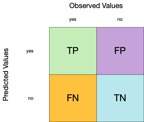
Confusion matrix

Confusion matrix
Confusion matrix

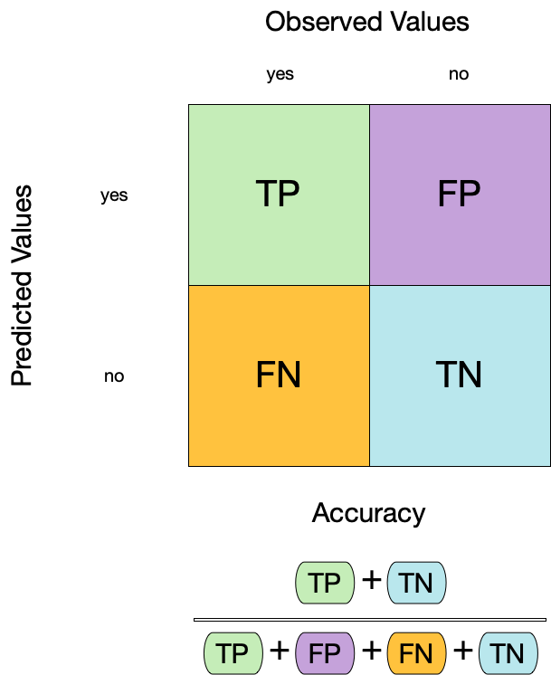
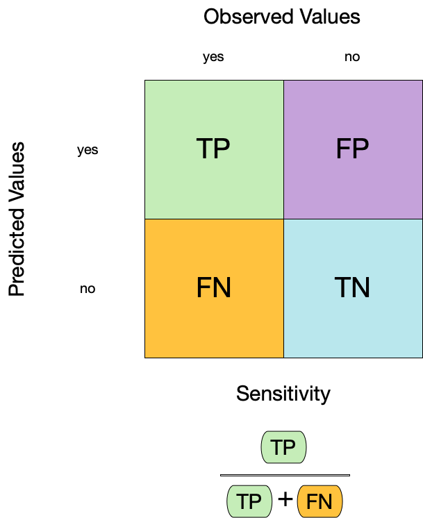
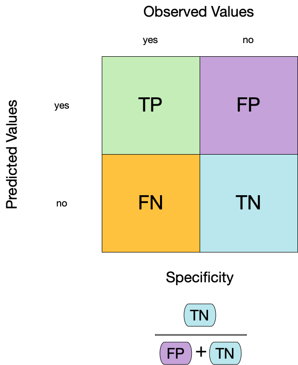
Metrics for model performance
Metrics for model performance
Metrics for model performance
Metrics for model performance
Metrics for model performance
We can use metric_set() to combine multiple calculations into one
forested_metrics <- metric_set(accuracy, specificity, sensitivity)
augment(forested_fit, new_data = forested_train) |>
forested_metrics(truth = forested, estimate = .pred_class)# A tibble: 3 × 3
.metric .estimator .estimate
<chr> <chr> <dbl>
1 accuracy binary 0.944
2 specificity binary 0.931
3 sensitivity binary 0.954Metrics for model performance
Metrics and metric sets work with grouped data frames!
augment(forested_fit, new_data = forested_train) |>
group_by(tree_no_tree) |>
accuracy(truth = forested, estimate = .pred_class)# A tibble: 2 × 4
tree_no_tree .metric .estimator .estimate
<fct> <chr> <chr> <dbl>
1 Tree accuracy binary 0.946
2 No tree accuracy binary 0.941Especially relevant for ML fairness assessment
⏱️ Your turn
Apply the forested_metrics metric set to augment()
output grouped by tree_no_tree.
Do any metrics differ substantially between groups?
02:00
augment(forested_fit, new_data = forested_train) |>
group_by(tree_no_tree) |>
forested_metrics(truth = forested, estimate = .pred_class)# A tibble: 6 × 4
tree_no_tree .metric .estimator .estimate
<fct> <chr> <chr> <dbl>
1 Tree accuracy binary 0.946
2 No tree accuracy binary 0.941
3 Tree specificity binary 0.582
4 No tree specificity binary 0.974
5 Tree sensitivity binary 0.984
6 No tree sensitivity binary 0.762Two class data
These metrics assume that we know the threshold for converting “soft” probability predictions into “hard” class predictions.
Is a 50% threshold good?
What happens if we say that we need to be 80% sure to declare an event?
- sensitivity ⬇️, specificity ⬆️
What happens for a 20% threshold?
- sensitivity ⬆️, specificity ⬇️
Varying the threshold

ROC curves
For an ROC (receiver operator characteristic) curve, we plot
- the false positive rate (1 - specificity) on the x-axis
- the true positive rate (sensitivity) on the y-axis
with sensitivity and specificity calculated at all possible thresholds.

ROC curves
We can use the area under the ROC curve as a classification metric:
- ROC AUC = 1 💯
- ROC AUC = 1/2 😢

ROC curves
# Assumes _first_ factor level is event; there are options to change that
augment(forested_fit, new_data = forested_train) |>
roc_curve(truth = forested, .pred_Yes) |>
slice(1, 20, 50)# A tibble: 3 × 3
.threshold specificity sensitivity
<dbl> <dbl> <dbl>
1 -Inf 0 1
2 0.235 0.885 0.972
3 0.909 0.969 0.826# A tibble: 1 × 3
.metric .estimator .estimate
<chr> <chr> <dbl>
1 roc_auc binary 0.975ROC curve plot
⏱️ Your turn
Compute and plot an ROC curve for the decision tree model.
What data are being used for this ROC curve plot?
03:00

Brier score
What if we don’t turn predicted probabilities into class predictions?
The Brier score is analogous to the mean squared error in regression models:
\[ Brier_{class} = \frac{1}{N}\sum_{i=1}^N\sum_{k=1}^C (y_{ik} - \hat{p}_{ik})^2 \]
Brier score
# A tibble: 1 × 3
.metric .estimator .estimate
<chr> <chr> <dbl>
1 brier_class binary 0.0469Smaller values are better, for binary classification the “bad model threshold” is about 0.25.
Separation vs calibration
The ROC captures separation.

The Brier score captures calibration.

⚠️ DANGERS OF OVERFITTING ⚠️
Dangers of overfitting

Illustration credit: https://github.com/topepo/2022-nyr-workshop/
Dangers of overfitting ⚠️

Illustration credit: https://github.com/topepo/2022-nyr-workshop/
Dangers of overfitting ⚠️
# A tibble: 5,685 × 22
.pred_class .pred_Yes .pred_No forested year elevation eastness northness
<fct> <dbl> <dbl> <fct> <dbl> <dbl> <dbl> <dbl>
1 No 0.0114 0.989 No 2016 464 -5 -99
2 Yes 0.636 0.364 Yes 2016 166 92 37
3 No 0.0114 0.989 No 2016 644 -85 -52
4 Yes 0.977 0.0226 Yes 2014 1285 4 99
5 Yes 0.977 0.0226 Yes 2013 822 87 48
6 Yes 0.808 0.192 Yes 2017 3 6 -99
7 Yes 0.977 0.0226 Yes 2014 2041 -95 28
8 Yes 0.977 0.0226 Yes 2015 1009 -8 99
9 No 0.0114 0.989 No 2017 436 -98 19
10 No 0.0114 0.989 No 2018 775 63 76
# ℹ 5,675 more rows
# ℹ 14 more variables: roughness <dbl>, tree_no_tree <fct>, dew_temp <dbl>,
# precip_annual <dbl>, temp_annual_mean <dbl>, temp_annual_min <dbl>,
# temp_annual_max <dbl>, temp_january_min <dbl>, vapor_min <dbl>,
# vapor_max <dbl>, canopy_cover <dbl>, lon <dbl>, lat <dbl>, land_type <fct>We call this “resubstitution” or “repredicting the training set”
Dangers of overfitting ⚠️
# A tibble: 1 × 3
  .metric  .estimator .estimate
  <chr>    <chr>          <dbl>
1 accuracy binary 0.944We call this a “resubstitution estimate”
Dangers of overfitting ⚠️
Dangers of overfitting ⚠️
⚠️ Remember that we’re demonstrating overfitting
⚠️ Don’t use the test set until the end of your modeling analysis
⏱️ Your turn
Use augment() and a metric function to compute a classification metric like brier_class().
Compute the metrics for both training and testing data to demonstrate overfitting!
Notice the evidence of overfitting! ⚠️
03:00
Dangers of overfitting ⚠️
What if we want to compare more models?
And/or more model configurations?
And we want to understand if these are important differences?
The testing data are precious 💎
How can we use the training data to compare and evaluate different models? 🤔
Cross-validation
Illustration credit: TMWR
Cross-validation
Illustration credit: TMWR
⏱️ Your turn
If we use 10 folds, what percent of the training data
- ends up in analysis
- ends up in assessment
for each fold?
01:00
Cross-validation
#  10-fold cross-validation
# A tibble: 10 × 2
   splits             id
   <list>             <chr>
 1 <split [5116/569]> Fold01
 2 <split [5116/569]> Fold02
 3 <split [5116/569]> Fold03
 4 <split [5116/569]> Fold04
 5 <split [5116/569]> Fold05
 6 <split [5117/568]> Fold06
 7 <split [5117/568]> Fold07
 8 <split [5117/568]> Fold08
 9 <split [5117/568]> Fold09
10 <split [5117/568]> Fold10
Cross-validation
What is in this?
Cross-validation
Cross-validation
We’ll use this setup:
#  10-fold cross-validation
# A tibble: 10 × 2
   splits             id
   <list>             <chr>
 1 <split [5116/569]> Fold01
 2 <split [5116/569]> Fold02
 3 <split [5116/569]> Fold03
 4 <split [5116/569]> Fold04
 5 <split [5116/569]> Fold05
 6 <split [5117/568]> Fold06
 7 <split [5117/568]> Fold07
 8 <split [5117/568]> Fold08
 9 <split [5117/568]> Fold09
10 <split [5117/568]> Fold10
Set the seed when creating resamples
We are equipped with metrics and resamples!
Fit our model to the resamples
# Resampling results
# 10-fold cross-validation
# A tibble: 10 × 4
   splits             id     .metrics         .notes
   <list>             <chr>  <list>           <list>
 1 <split [5116/569]> Fold01 <tibble [3 × 4]> <tibble [0 × 3]>
 2 <split [5116/569]> Fold02 <tibble [3 × 4]> <tibble [0 × 3]>
 3 <split [5116/569]> Fold03 <tibble [3 × 4]> <tibble [0 × 3]>
 4 <split [5116/569]> Fold04 <tibble [3 × 4]> <tibble [0 × 3]>
 5 <split [5116/569]> Fold05 <tibble [3 × 4]> <tibble [0 × 3]>
 6 <split [5117/568]> Fold06 <tibble [3 × 4]> <tibble [0 × 3]>
 7 <split [5117/568]> Fold07 <tibble [3 × 4]> <tibble [0 × 3]>
 8 <split [5117/568]> Fold08 <tibble [3 × 4]> <tibble [0 × 3]>
 9 <split [5117/568]> Fold09 <tibble [3 × 4]> <tibble [0 × 3]>
10 <split [5117/568]> Fold10 <tibble [3 × 4]> <tibble [0 × 3]>
Evaluating model performance
# A tibble: 3 × 6
  .metric     .estimator   mean     n std_err .config
  <chr>       <chr>       <dbl> <int>   <dbl> <chr>
1 accuracy    binary     0.894     10 0.00562 Preprocessor1_Model1
2 brier_class binary     0.0817    10 0.00434 Preprocessor1_Model1
3 roc_auc binary 0.951 10 0.00378 Preprocessor1_Model1We can reliably measure performance using only the training data 🎉
Comparing metrics
How do the metrics from resampling compare to the metrics from training and testing?
The ROC AUC previously was
- 0.97 for the training set
- 0.95 for test set
Remember that:
⚠️ the training set gives you overly optimistic metrics
⚠️ the test set is precious
Evaluating model performance
# Save the assessment set results
ctrl_forested <- control_resamples(save_pred = TRUE)
forested_res <- fit_resamples(forested_wflow, forested_folds, control = ctrl_forested)

forested_res
# Resampling results
# 10-fold cross-validation
# A tibble: 10 × 5
splits id .metrics .notes .predictions
<list> <chr> <list> <list> <list>
1 <split [5116/569]> Fold01 <tibble [3 × 4]> <tibble [0 × 3]> <tibble>
2 <split [5116/569]> Fold02 <tibble [3 × 4]> <tibble [0 × 3]> <tibble>
3 <split [5116/569]> Fold03 <tibble [3 × 4]> <tibble [0 × 3]> <tibble>
4 <split [5116/569]> Fold04 <tibble [3 × 4]> <tibble [0 × 3]> <tibble>
5 <split [5116/569]> Fold05 <tibble [3 × 4]> <tibble [0 × 3]> <tibble>
6 <split [5117/568]> Fold06 <tibble [3 × 4]> <tibble [0 × 3]> <tibble>
7 <split [5117/568]> Fold07 <tibble [3 × 4]> <tibble [0 × 3]> <tibble>
8 <split [5117/568]> Fold08 <tibble [3 × 4]> <tibble [0 × 3]> <tibble>
9 <split [5117/568]> Fold09 <tibble [3 × 4]> <tibble [0 × 3]> <tibble>
10 <split [5117/568]> Fold10 <tibble [3 × 4]> <tibble [0 × 3]> <tibble> Evaluating model performance
# Save the assessment set results
forested_preds <- collect_predictions(forested_res)
forested_preds# A tibble: 5,685 × 7
.pred_class .pred_Yes .pred_No id .row forested .config
<fct> <dbl> <dbl> <chr> <int> <fct> <chr>
1 Yes 0.5 0.5 Fold01 2 Yes Preprocessor1_Model1
2 Yes 0.982 0.0178 Fold01 5 Yes Preprocessor1_Model1
3 No 0.00790 0.992 Fold01 9 No Preprocessor1_Model1
4 No 0.4 0.6 Fold01 14 No Preprocessor1_Model1
5 Yes 0.870 0.130 Fold01 18 Yes Preprocessor1_Model1
6 Yes 0.982 0.0178 Fold01 59 Yes Preprocessor1_Model1
7 No 0.00790 0.992 Fold01 67 No Preprocessor1_Model1
8 Yes 0.982 0.0178 Fold01 89 Yes Preprocessor1_Model1
9 No 0.00790 0.992 Fold01 94 No Preprocessor1_Model1
10 Yes 0.982 0.0178 Fold01 111 Yes Preprocessor1_Model1
# ℹ 5,675 more rowsEvaluating model performance
# A tibble: 30 × 4
id .metric .estimator .estimate
<chr> <chr> <chr> <dbl>
1 Fold01 accuracy binary 0.896
2 Fold02 accuracy binary 0.859
3 Fold03 accuracy binary 0.868
4 Fold04 accuracy binary 0.921
5 Fold05 accuracy binary 0.900
6 Fold06 accuracy binary 0.891
7 Fold07 accuracy binary 0.896
8 Fold08 accuracy binary 0.903
9 Fold09 accuracy binary 0.896
10 Fold10 accuracy binary 0.905
# ℹ 20 more rowsWhere are the fitted models?
# Resampling results
# 10-fold cross-validation
# A tibble: 10 × 5
   splits             id     .metrics         .notes           .predictions
   <list>             <chr>  <list>           <list>           <list>
 1 <split [5116/569]> Fold01 <tibble [3 × 4]> <tibble [0 × 3]> <tibble>
 2 <split [5116/569]> Fold02 <tibble [3 × 4]> <tibble [0 × 3]> <tibble>
 3 <split [5116/569]> Fold03 <tibble [3 × 4]> <tibble [0 × 3]> <tibble>
 4 <split [5116/569]> Fold04 <tibble [3 × 4]> <tibble [0 × 3]> <tibble>
 5 <split [5116/569]> Fold05 <tibble [3 × 4]> <tibble [0 × 3]> <tibble>
 6 <split [5117/568]> Fold06 <tibble [3 × 4]> <tibble [0 × 3]> <tibble>
 7 <split [5117/568]> Fold07 <tibble [3 × 4]> <tibble [0 × 3]> <tibble>
 8 <split [5117/568]> Fold08 <tibble [3 × 4]> <tibble [0 × 3]> <tibble>
 9 <split [5117/568]> Fold09 <tibble [3 × 4]> <tibble [0 × 3]> <tibble>
10 <split [5117/568]> Fold10 <tibble [3 × 4]> <tibble [0 × 3]> <tibble> 🗑️️
A side quest on bias vs. variance
Bias vs. variance
- Bias - degree to which something deviates from its true underlying value
- Variance - degree to which values can fluctuate
Extended discussion: Feature Engineering and Selection
Classic bulls-eye example

Bias-variance trade-off in ML
High variance: small changes to underlying data cause a sizable change in the model parameters/structure
- Decision trees
- Nearest neighbors
- Neural networks
Low variance: model is stable across different datasets
- Linear regression
- Logistic regression
- Partial least squares
High bias: model is unable to predict values close to the true value
- Linear regression
- Logistic regression
- Partial least squares
Low bias: model is highly flexible and has capacity to fit a variety of shapes and patterns
- Decision trees
- Nearest neighbors
- Neural networks
Bias-variance trade-off in ML

Bias-variance trade-off in ML

Bias-variance trade-off in ML

Why does this matter to resampling?
- Resampling methods also introduce an element of bias and variance
- Variance: how much do the metrics change when we change the resampling procedure?
- Bias: ability of a resampling scheme to be able to hit the true underlying performance metric1
In general terms,
- As sample size for assessment increases, bias decreases
- As the number of resamples increases, variance decreases
Different resampling methods have different bias-variance trade-offs
Alternate resampling schemes
Repeated cross-validation
- \(V\) - number of partitions
- \(R\) - number of repetitions of the partitioning process
- More resamples, lower variance (but longer compute time)
#  10-fold cross-validation repeated 5 times
# A tibble: 50 × 3
   splits             id      id2
   <list>             <chr>   <chr>
 1 <split [5116/569]> Repeat1 Fold01
 2 <split [5116/569]> Repeat1 Fold02
 3 <split [5116/569]> Repeat1 Fold03
 4 <split [5116/569]> Repeat1 Fold04
 5 <split [5116/569]> Repeat1 Fold05
 6 <split [5117/568]> Repeat1 Fold06
 7 <split [5117/568]> Repeat1 Fold07
 8 <split [5117/568]> Repeat1 Fold08
 9 <split [5117/568]> Repeat1 Fold09
10 <split [5117/568]> Repeat1 Fold10
# ℹ 40 more rows
Monte Carlo Cross-Validation
- Allocate fixed proportion of data to the assessment sets
- Proportion of data selected for assessment is random with each fold (i.e. assessment sets are not mutually exclusive)
- Benefits to be demonstrated…
# Monte Carlo cross-validation (0.75/0.25) with 10 resamples
# A tibble: 10 × 2
   splits              id
   <list>              <chr>
 1 <split [4263/1422]> Resample01
 2 <split [4263/1422]> Resample02
 3 <split [4263/1422]> Resample03
 4 <split [4263/1422]> Resample04
 5 <split [4263/1422]> Resample05
 6 <split [4263/1422]> Resample06
 7 <split [4263/1422]> Resample07
 8 <split [4263/1422]> Resample08
 9 <split [4263/1422]> Resample09
10 <split [4263/1422]> Resample10
Bootstrapping
Illustration credit: https://www.tmwr.org/resampling
Bootstrapping
- Resamples the same size as the training set drawn with replacement
# Bootstrap sampling
# A tibble: 25 × 2
   splits              id
   <list>              <chr>
 1 <split [5685/2075]> Bootstrap01
 2 <split [5685/2093]> Bootstrap02
 3 <split [5685/2129]> Bootstrap03
 4 <split [5685/2093]> Bootstrap04
 5 <split [5685/2111]> Bootstrap05
 6 <split [5685/2105]> Bootstrap06
 7 <split [5685/2139]> Bootstrap07
 8 <split [5685/2079]> Bootstrap08
 9 <split [5685/2113]> Bootstrap09
10 <split [5685/2101]> Bootstrap10
# ℹ 15 more rows
Validation set
Illustration credit: https://www.tmwr.org/resampling
Validation set
- Popular for large datasets and highly computationally-intensive models
A validation set is just another type of resample
The whole game - status update

Decision tree 🌳
Random forest 🌳🌲🌴🌵🌴🌳🌳🌴🌲🌵🌴🌲🌳🌴🌳🌵🌵🌴🌲🌲🌳🌴🌳🌴🌲🌴🌵🌴🌲🌴🌵🌲🌵🌴🌲🌳🌴🌵🌳🌴🌳
Random forest 🌳🌲🌴🌵🌳🌳🌴🌲🌵🌴🌳🌵
Ensemble many decision tree models
All the trees vote! 🗳️
Bootstrap aggregating + random predictor sampling
- Often works well without tuning hyperparameters (more on this later!), as long as there are enough trees
Create a random forest model
Create a random forest model
══ Workflow ══════════════════════════════════════════════════════════
Preprocessor: Formula
Model: rand_forest()
── Preprocessor ──────────────────────────────────────────────────────
forested ~ .
── Model ─────────────────────────────────────────────────────────────
Random Forest Model Specification (classification)

Main Arguments:
  trees = 1000

Computational engine: ranger ⏱️ Your turn
Use fit_resamples() and rf_wflow to:
- keep predictions
- compute metrics
08:00
Evaluating model performance
ctrl_forested <- control_resamples(save_pred = TRUE)
# Random forest uses random numbers so set the seed first
set.seed(234)
rf_res <- fit_resamples(rf_wflow, forested_folds, control = ctrl_forested)
collect_metrics(rf_res)# A tibble: 3 × 6
.metric .estimator mean n std_err .config
<chr> <chr> <dbl> <int> <dbl> <chr>
1 accuracy binary 0.918 10 0.00563 Preprocessor1_Model1
2 brier_class binary 0.0616 10 0.00338 Preprocessor1_Model1
3 roc_auc binary 0.972 10 0.00308 Preprocessor1_Model1The whole game - status update

The final fit
Suppose that we are happy with our random forest model.
Let’s fit the model on the training set and verify our performance using the test set.
We’ve shown you fit() and predict() (+ augment()) but there is a shortcut:
# Resampling results
# Manual resampling
# A tibble: 1 × 6
splits id .metrics .notes .predictions .workflow
<list> <chr> <list> <list> <list> <list>
1 <split [5685/1422]> train/test split <tibble> <tibble> <tibble> <workflow>What is in final_fit?
# A tibble: 3 × 4
.metric .estimator .estimate .config
<chr> <chr> <dbl> <chr>
1 accuracy binary 0.910 Preprocessor1_Model1
2 roc_auc binary 0.970 Preprocessor1_Model1
3 brier_class binary 0.0652 Preprocessor1_Model1These are metrics computed with the test set
What is in final_fit?
# A tibble: 1,422 × 7
.pred_class .pred_Yes .pred_No id .row forested .config
<fct> <dbl> <dbl> <chr> <int> <fct> <chr>
1 Yes 0.835 0.165 train/test split 3 No Preprocessor1…
2 Yes 0.726 0.274 train/test split 4 Yes Preprocessor1…
3 No 0.289 0.711 train/test split 7 Yes Preprocessor1…
4 Yes 0.534 0.466 train/test split 8 Yes Preprocessor1…
5 Yes 0.554 0.446 train/test split 10 Yes Preprocessor1…
6 Yes 0.978 0.0225 train/test split 11 Yes Preprocessor1…
7 Yes 0.968 0.0322 train/test split 12 Yes Preprocessor1…
8 Yes 0.963 0.0373 train/test split 14 Yes Preprocessor1…
9 Yes 0.944 0.0563 train/test split 15 Yes Preprocessor1…
10 Yes 0.981 0.0188 train/test split 19 Yes Preprocessor1…
# ℹ 1,412 more rowsWhat is in final_fit?
══ Workflow [trained] ════════════════════════════════════════════════
Preprocessor: Formula
Model: rand_forest()
── Preprocessor ──────────────────────────────────────────────────────
forested ~ .
── Model ─────────────────────────────────────────────────────────────
Ranger result
Call:
ranger::ranger(x = maybe_data_frame(x), y = y, num.trees = ~1000, num.threads = 1, verbose = FALSE, seed = sample.int(10^5, 1), probability = TRUE)
Type: Probability estimation
Number of trees: 1000
Sample size: 5685
Number of independent variables: 18
Mtry: 4
Target node size: 10
Variable importance mode: none
Splitrule: gini
OOB prediction error (Brier s.): 0.06164335 Use this for prediction on new data, like for deploying
The whole game

Tuning
Tuning parameters
Some model or preprocessing parameters cannot be estimated directly from the data.
Some examples:
- Tree depth in decision trees
- Number of neighbors in a K-nearest neighbor model
- Learning rate in a gradient boosting model
- Number of knots in a spline function
Optimize tuning parameters
- Try different values and measure their performance.
- Find good values for these parameters.
- Once the value(s) of the parameter(s) are determined, a model can be finalized by fitting the model to the entire training set.
Optimize tuning parameters
The main two strategies for optimization are:
Grid search 💠 which tests a pre-defined set of candidate values
Iterative search 🌀 which suggests/estimates new values of candidate parameters to evaluate
Specifying tuning parameters
Let’s take our previous random forest workflow and tag for tuning the minimum number of data points in each node:
rf_spec <- rand_forest(min_n = tune()) |>
set_mode("classification")
rf_wflow <- workflow(forested ~ ., rf_spec)
rf_wflow
══ Workflow ══════════════════════════════════════════════════════════
Preprocessor: Formula
Model: rand_forest()
── Preprocessor ──────────────────────────────────────────────────────
forested ~ .
── Model ─────────────────────────────────────────────────────────────
Random Forest Model Specification (classification)
Main Arguments:
min_n = tune()
Computational engine: ranger Try out multiple values
tune_grid() works similar to fit_resamples() but covers multiple parameter values:
Compare results
Inspecting results and selecting the best-performing hyperparameter(s):
# A tibble: 5 × 7
  min_n .metric .estimator  mean     n std_err .config
  <int> <chr>   <chr>      <dbl> <int>   <dbl> <chr>
1    21 roc_auc binary     0.972    10 0.00295 Preprocessor1_Model4
2     6 roc_auc binary     0.972    10 0.00303 Preprocessor1_Model2
3    31 roc_auc binary     0.972    10 0.00317 Preprocessor1_Model3
4    13 roc_auc binary     0.972    10 0.00311 Preprocessor1_Model5
5 33 roc_auc binary 0.972 10 0.00322 Preprocessor1_Model1# A tibble: 1 × 2
min_n .config
<int> <chr>
1 21 Preprocessor1_Model4collect_metrics() and autoplot() are also available.
The final fit
rf_wflow <- finalize_workflow(rf_wflow, best_parameter)

final_fit <- last_fit(rf_wflow, forested_split)

collect_metrics(final_fit)
# A tibble: 3 × 4
.metric .estimator .estimate .config
<chr> <chr> <dbl> <chr>
1 accuracy binary 0.906 Preprocessor1_Model1
2 roc_auc binary 0.970 Preprocessor1_Model1
3 brier_class binary 0.0656 Preprocessor1_Model1⏱️ Your turn
Modify your model workflow to tune one or more parameters.
Use grid search to find the best parameter(s).
05:00
Wrap-up
Recap
- Classification metrics can be used to evaluate model performance, including hard and soft predictions
- Overfitting can be detected by comparing training and testing metrics
- Cross-validation is a powerful tool for comparing models
- Random forests are an ensemble of decision trees
- Tuning parameters can be optimized using grid search
Acknowledgments
- Materials derived in part from Machine learning with {tidymodels} and licensed under a Creative Commons Attribution-ShareAlike 4.0 International (CC BY-SA) License.
My latest school tax bill


