Tune your workflows
Lecture 7
Cornell University
INFO 4940/5940 - Fall 2025
September 16, 2025
Announcements
Homework 01 recap
Submit a rendered PDF to Gradescope
Review the Quarto tutorials
Code comments document what the code does:
Text content is used explain or interpret the results of your output
The random forest model was not great. The RMSE was much lower than the linear regression model in the previous exercise.
Document your code
Review the suggested solution keys to ensure you are following best practices
Homework 02 due tomorrow
Learning objectives
- Define tuning parameters for machine learning models
- Introduce boosted trees models
- Utilize grid search to optimize tuning parameters
- Implement space-filling designs for grid searches
- Introduce iterative search procedures for tuning parameters
- Finalize the model for production
From last time
Previously - data partition
Optimizing models via tuning parameters
Tuning parameters
Model parameters - configuration settings that are estimated from the data during model fitting.
Tuning parameters - configuration settings that are set prior to model fitting and whose values are not estimated from the data
Also known as hyperparameters
📝 Is this a tuning parameter?
Identify if the following are tuning parameters
✅ Learning rate in a boosted tree model
❌ Coefficients in a linear regression model
✅ Number of neighbors in a K-nearest neighbor model
✅ Number of knots in a spline basis expansion
❌ Weights in a neural network
❌ The random seed used to initialize the model fitting
Tuning parameters can be anywhere in the model workflow (preprocessing or model specification).
03:00
Optimize tuning parameters
- Try different values and measure their performance
- Find good values for these parameters
- Once the value(s) of the parameter(s) are determined, a model can be finalized by fitting the model to the entire training set using the chosen parameter values
Optimizing a model
holidays <- c(
  "AllSouls",
  "AshWednesday",
  "ChristmasEve",
  "Easter",
  "ChristmasDay",
  "GoodFriday",
  "NewYearsDay",
  "PalmSunday"
)

basic_rec <- recipe(avg_price_per_room ~ ., data = hotel_train) |>
  step_YeoJohnson(lead_time) |>
  step_date(arrival_date) |>
  step_holiday(arrival_date, holidays = holidays) |>
  step_rm(arrival_date) |>
  step_zv(all_predictors())
We will use a tree-based model in a minute.
- The categorical predictors are left as-is
- That’s why there is no
step_dummy()
Ensemble tree-based methods
Ensemble methods
Ensemble methods combine many simple “building block” models in order to obtain a single and potentially very powerful model.
- Individual models are typically weak learners - low accuracy on their own
- Combining a set of weak learners can create a strong learner with high accuracy by reducing bias and variance
Bagging
Decision trees suffer from high variance - small changes in the data can lead to very different trees
Bootstrap aggregation (or bagging) reduces the variance of a model by averaging the predictions of many models trained on different samples (with replacement) of the data.
Random forests
To further improve performance over bagged trees, random forests introduce additional randomness in the model-building process to reduce the correlation across the trees.
- Random feature selection: At each split, only a random subset of features are considered
- Makes each individual model simpler (and “dumber”), but improves the overall performance of the forest
Boosting
Unlike bagging and random forests, which build trees independently, boosting builds trees sequentially, with each new tree trying to correct the errors of the previous trees.
How do you study?
Slow, methodical preparation

Cram the night before

Which is more effective in the long run? Learning slowly
Boosted trees
- Fit a decision tree to the residuals from the model
- Add the tree to the model and update the residuals
- Repeat steps 1 and 2 until complete
Each tree is small - only a handful of terminal nodes
Each tree uses the results of the previous tree to better predict samples, especially those that have been poorly predicted.
Each tree in the ensemble is saved and new samples are predicted using a weighted average of the votes of each tree in the ensemble.
Popular implementations
- Adaboost (Adaptive Boosting)
- Gradient boosting
- LightGBM (Light Gradient Boosting Machine)
- XGBoost (Extreme Gradient Boosting)
Boosted tree tuning parameters
Some possible parameters:
mtry: The number of predictors randomly sampled at each split (in \([1, \text{ncol}(x)]\) or \((0, 1]\)).min_n: The number of samples needed to further split (\([1, n]\)).learn_rate: The rate that each tree adapts from previous iterations (\((0, \infty]\), usual maximum is 0.1).trees: The number of trees (\([1, \infty]\), but usually up to thousands)stop_iter: The number of iterations of boosting where no improvement was shown before stopping (\([1, trees]\))
min_n
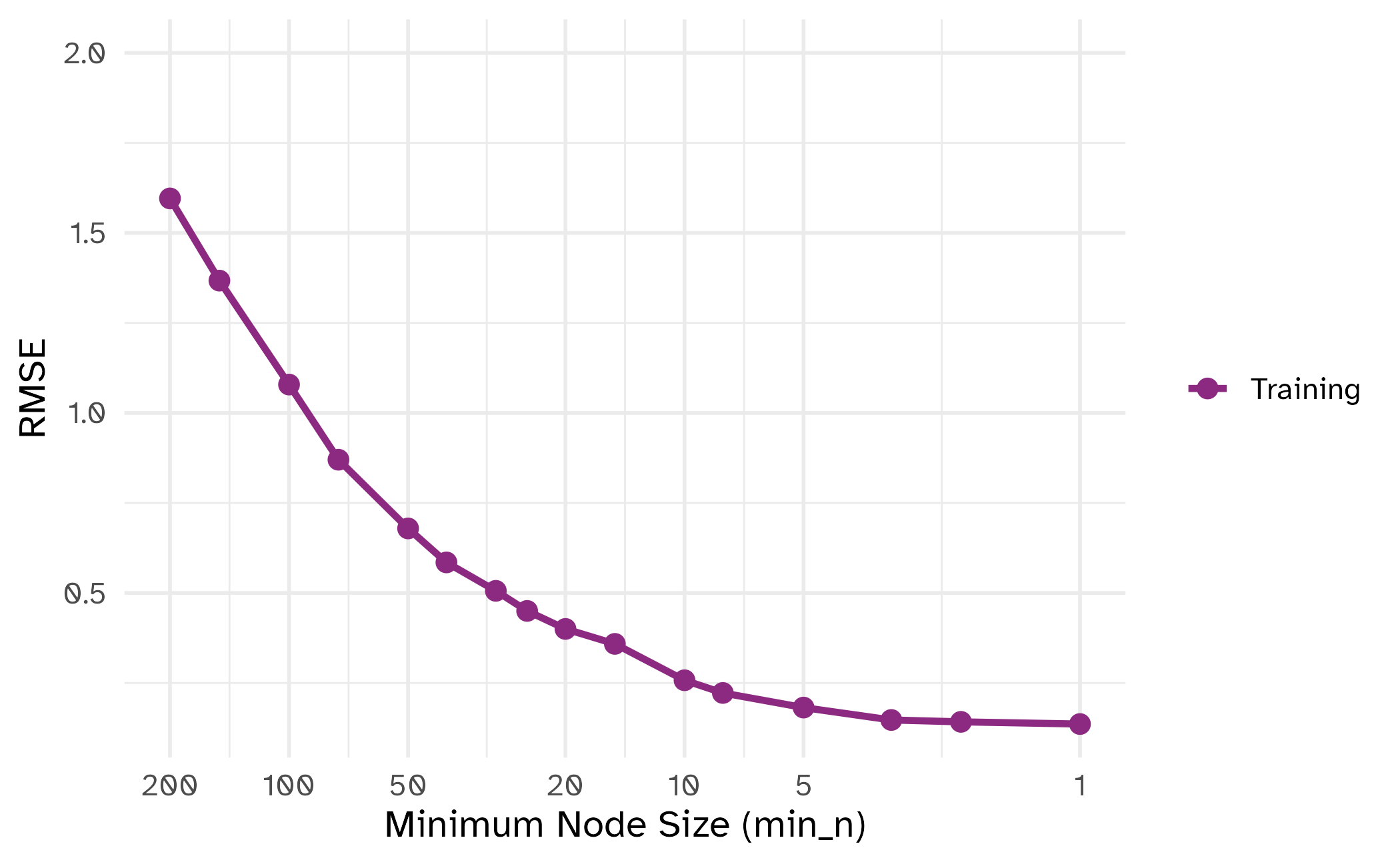
min_n
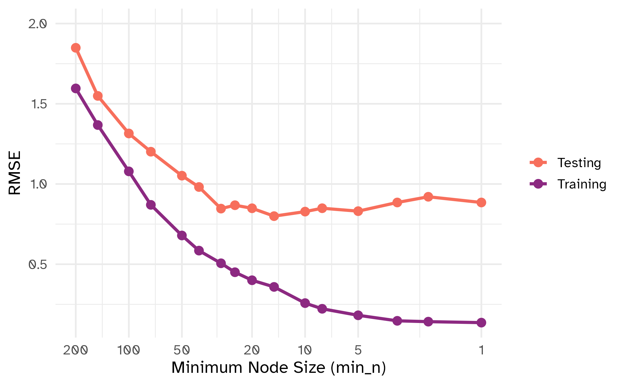
Recap: boosted trees tuning parameters
| tuning parameter | overfit? |
|---|---|
min_n |
⬇️ |
learn_rate
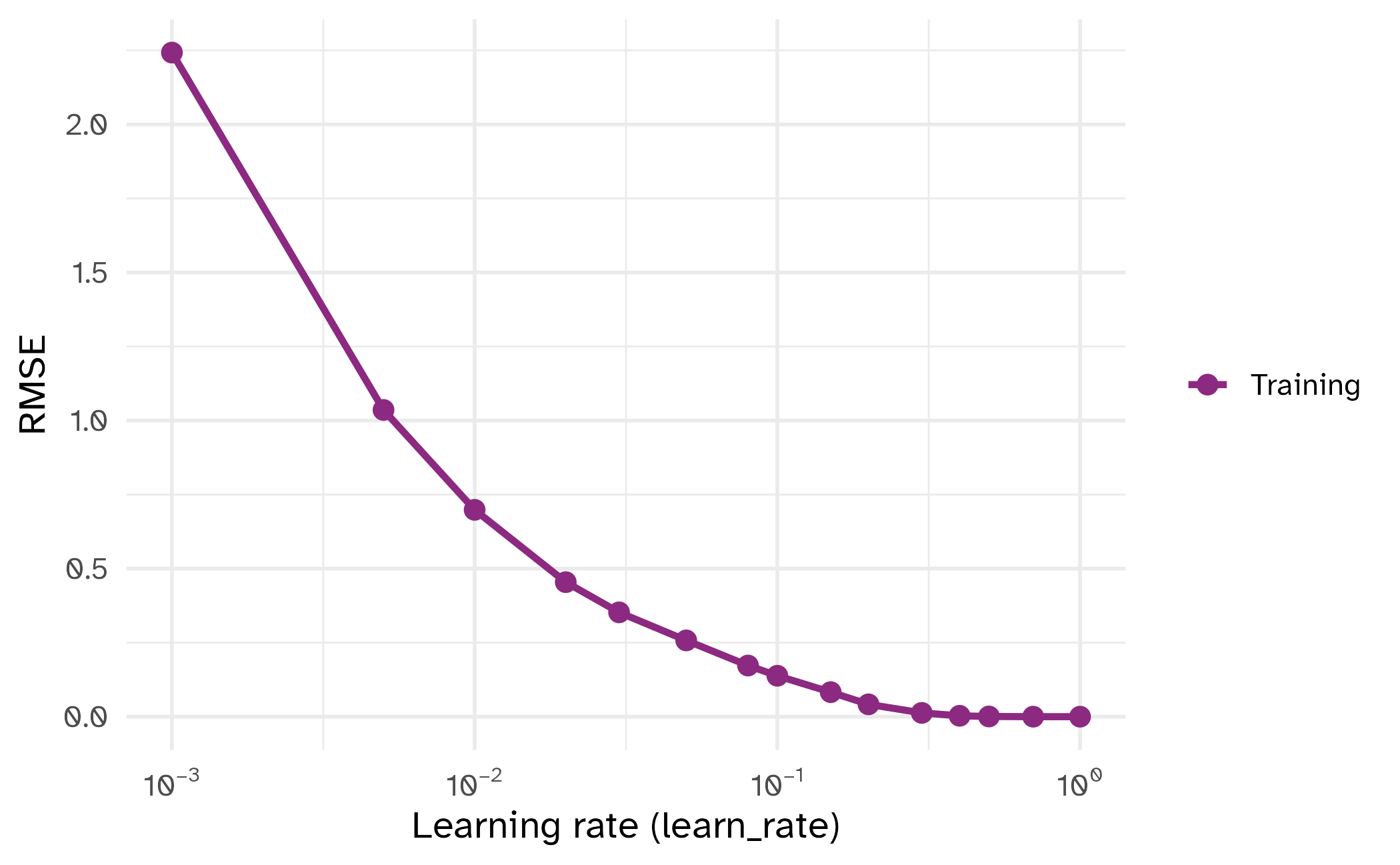
learn_rate
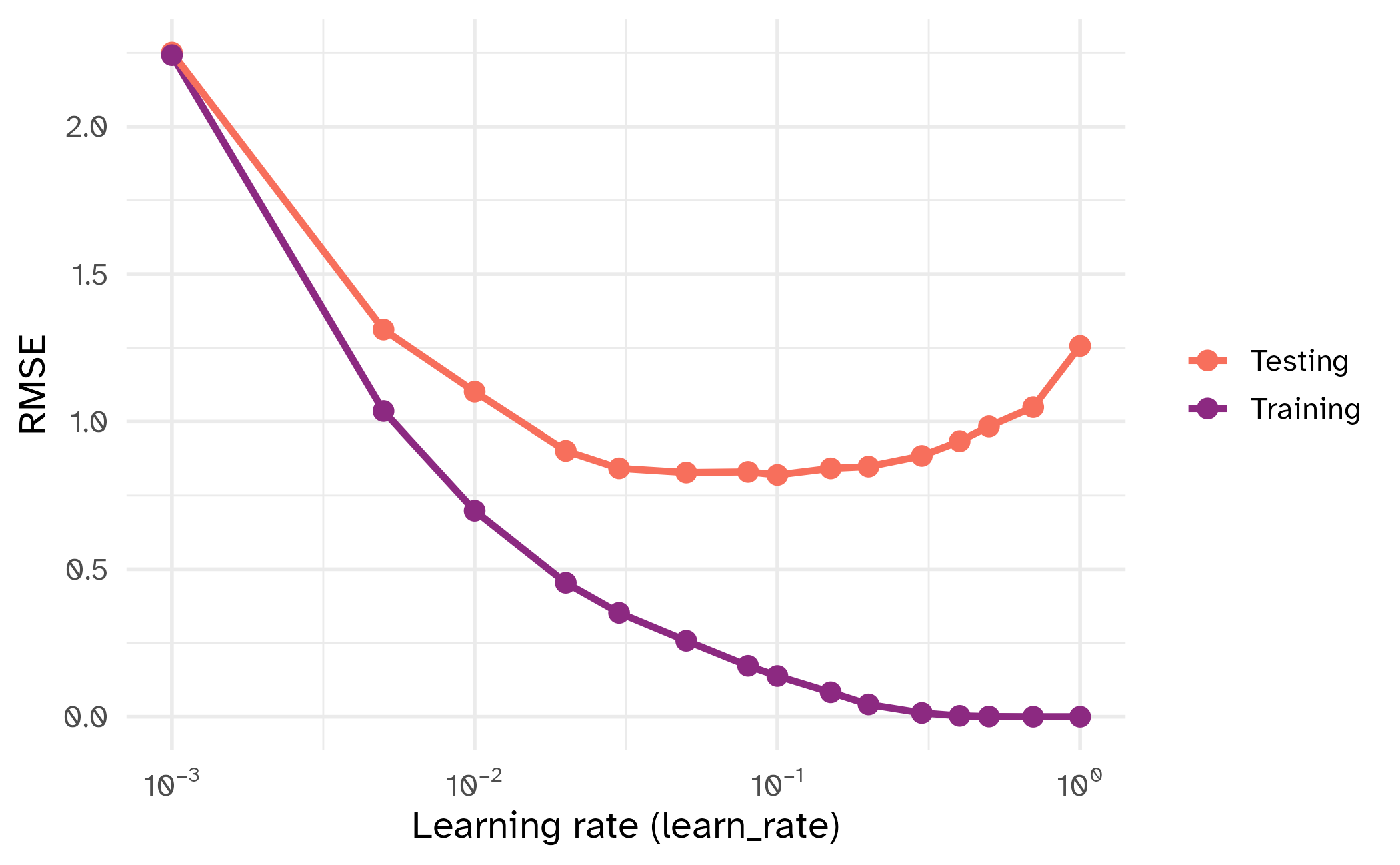
Recap: boosted trees tuning parameters
| tuning parameter | overfit? |
|---|---|
min_n |
⬇️ |
learn_rate |
⬆️ |
Boosted tree tuning parameters
It is usually not difficult to optimize these models.
Often, there are multiple candidate tuning parameter combinations that have very good results.
To demonstrate simple concepts, we’ll look at optimizing the number of trees in the ensemble (between 1 and 100) and the learning rate (\(10^{-5}\) to \(10^{-1}\)).
Boosted tree tuning parameters
Light GBM implemented using lightgbm package. Uses its own syntax for fitting models, but also includes a scikit-learn compatible API.
Optimize tuning parameters
The main two strategies for optimization are:
Grid search 💠 which tests a pre-defined set of candidate values
Iterative search 🌀 which suggests/estimates new values of candidate parameters to evaluate
Grid search
A small grid of points trying to minimize the error via learning rate:

Grid search
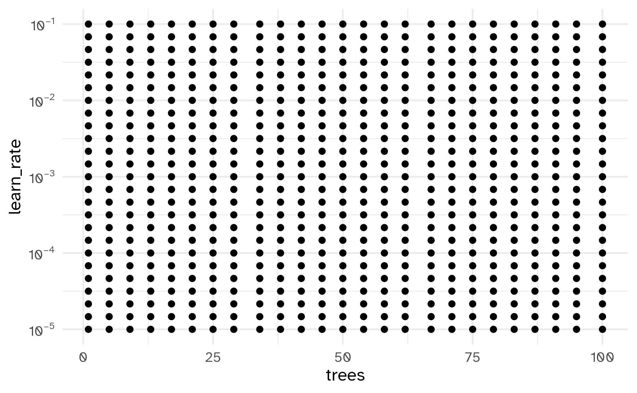
In reality we would probably sample the space more densely:

Iterative search
We could start with a few points and search the space:
Grid search
Different types of grids
Different types of grids
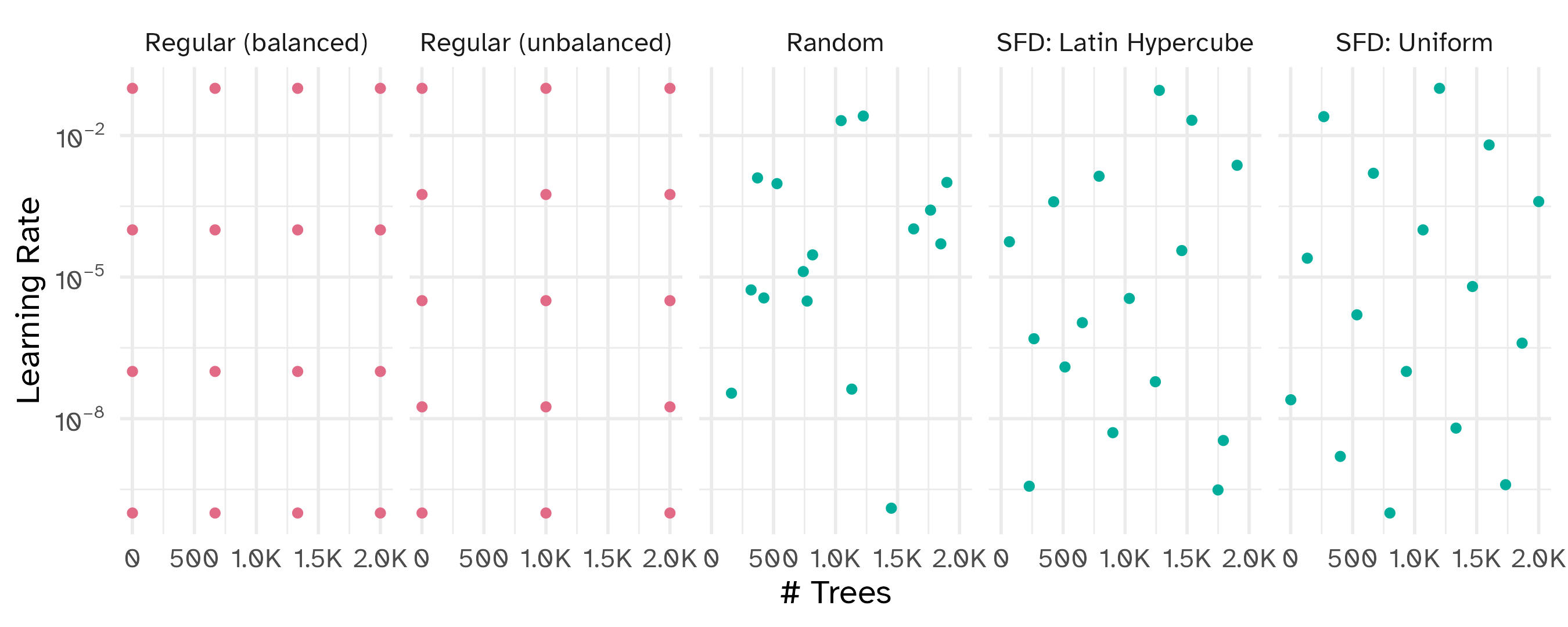
Space-filling designs (SFD) attempt to cover the parameter space without redundant candidates.
Create a regular grid manually
# A tibble: 16 × 2
   trees learn_rate
   <dbl>      <dbl>
 1     1   0.00001
 2     1   0.000215
 3     1   0.00464
 4     1   0.1
 5    34   0.00001
 6    34   0.000215
 7    34   0.00464
 8    34   0.1
 9    67   0.00001
10    67   0.000215
11    67   0.00464
12    67   0.1
13   100   0.00001
14   100   0.000215
15   100   0.00464
16   100   0.1
Create your tuning grid as a dictionary with parameter names as keys and lists of candidate values as values.
Create a grid
Collection of 2 parameters for tuning identifier type object
trees trees nparam[+]
learn_rate learn_rate nparam[+]# Trees (quantitative)Range: [1, 2000]Learning Rate (quantitative)Transformer: log-10 [1e-100, Inf]Range (transformed scale): [-10, -1]Create a grid automatically
# A tibble: 25 × 2
   trees learn_rate
   <int>      <dbl>
 1     1   1.78e- 5
 2    84   4.22e- 8
 3   167   3.16e- 3
 4   250   5.62e-10
 5   334   1.33e- 6
 6   417   1   e- 4
 7   500   1.78e- 2
 8   584   1.78e- 8
 9   667   2.37e-10
10   750   3.16e- 6
# ℹ 15 more rows
Create a regular grid
# A tibble: 16 × 2
   trees   learn_rate
   <int>        <dbl>
 1     1 0.0000000001
 2   667 0.0000000001
 3  1333 0.0000000001
 4  2000 0.0000000001
 5     1 0.0000001
 6   667 0.0000001
 7  1333 0.0000001
 8  2000 0.0000001
 9     1 0.0001
10   667 0.0001
11  1333 0.0001
12  2000 0.0001
13     1 0.1
14   667 0.1
15  1333 0.1
16  2000 0.1
📝 Regular vs. irregular tuning grids
Identify for each scenario which type of grid is more appropriate
| Scenario | Potential values | Regular | Space-filling |
|---|---|---|---|
| Number of tuning parameters | Low/high | Low | High |
| Prior knowledge of tuning parameters | Unknown/known ranges | Known ranges | Unknown ranges |
| Computational budget | Limited/ample | Ample | Limited |
| Interpretability needs | Low/high | High | Low |
04:00
Update parameter ranges
Often you will want to manually set the ranges of the tuning parameters.
# A tibble: 625 × 2
   trees learn_rate
   <int>      <dbl>
 1     1    0.00001
 2     5    0.00001
 3     9    0.00001
 4    13    0.00001
 5    17    0.00001
 6    21    0.00001
 7    25    0.00001
 8    29    0.00001
 9    34    0.00001
10    38    0.00001
# ℹ 615 more rows
The results
Choosing tuning parameters
Let’s take our previous model and tune more parameters:
Grid search
Grid search
# Tuning results
# 10-fold cross-validation using stratification
# A tibble: 10 × 5
   splits             id     .metrics          .notes           .predictions
   <list>             <chr>  <list>            <list>           <list>
 1 <split [3372/377]> Fold01 <tibble [50 × 7]> <tibble [0 × 3]> <tibble [9,425 × 7]>
 2 <split [3373/376]> Fold02 <tibble [50 × 7]> <tibble [0 × 3]> <tibble [9,400 × 7]>
 3 <split [3373/376]> Fold03 <tibble [50 × 7]> <tibble [0 × 3]> <tibble [9,400 × 7]>
 4 <split [3373/376]> Fold04 <tibble [50 × 7]> <tibble [0 × 3]> <tibble [9,400 × 7]>
 5 <split [3373/376]> Fold05 <tibble [50 × 7]> <tibble [0 × 3]> <tibble [9,400 × 7]>
 6 <split [3374/375]> Fold06 <tibble [50 × 7]> <tibble [0 × 3]> <tibble [9,375 × 7]>
 7 <split [3375/374]> Fold07 <tibble [50 × 7]> <tibble [0 × 3]> <tibble [9,350 × 7]>
 8 <split [3376/373]> Fold08 <tibble [50 × 7]> <tibble [0 × 3]> <tibble [9,325 × 7]>
 9 <split [3376/373]> Fold09 <tibble [50 × 7]> <tibble [0 × 3]> <tibble [9,325 × 7]>
10 <split [3376/373]> Fold10 <tibble [50 × 7]> <tibble [0 × 3]> <tibble [9,325 × 7]>
Grid results
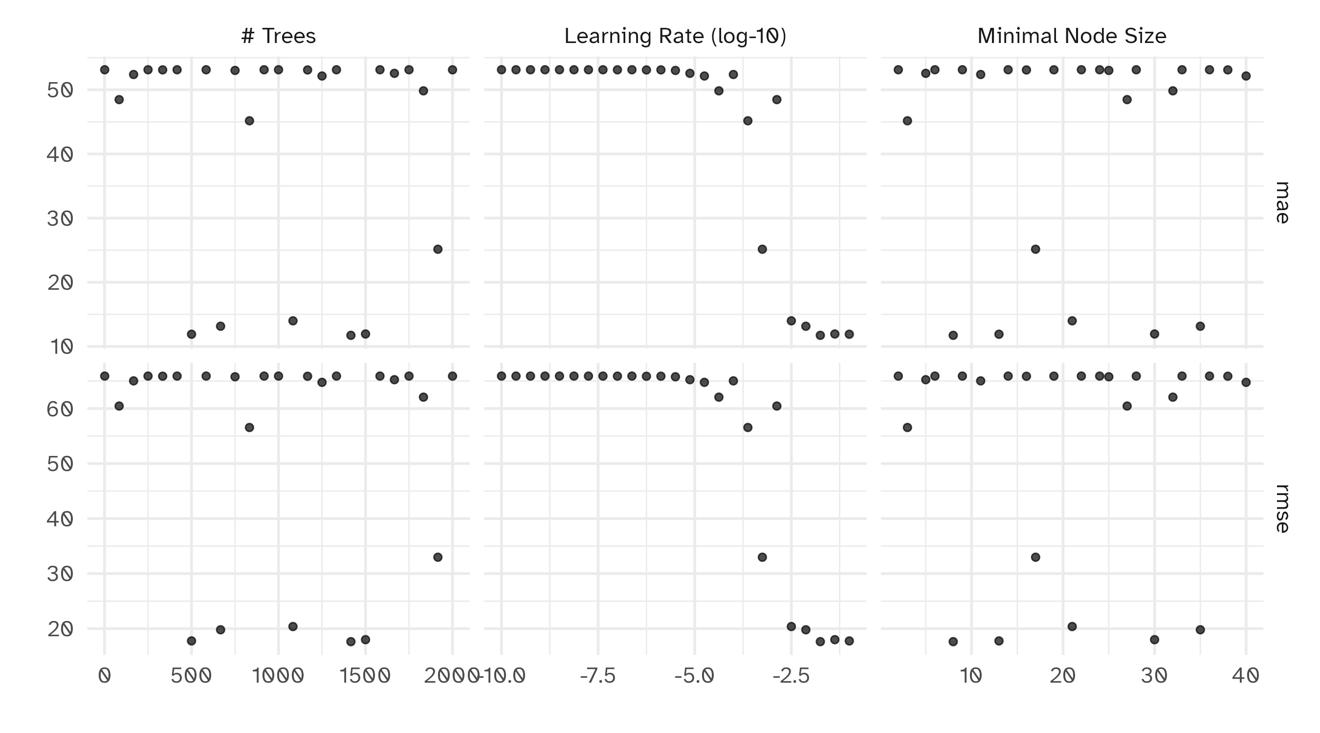
Tuning results
# A tibble: 50 × 9
   trees min_n   learn_rate .metric .estimator  mean     n std_err .config
   <int> <int>        <dbl> <chr>   <chr>      <dbl> <int>   <dbl> <chr>
 1   917     2 0.0000000178 mae     standard    53.1    10   0.306 Preprocessor1_Model01
 2   917     2 0.0000000178 rmse    standard    65.9    10   0.561 Preprocessor1_Model01
 3   833     3 0.000237     mae     standard    45.2    10   0.245 Preprocessor1_Model02
 4   833     3 0.000237     rmse    standard    56.6    10   0.492 Preprocessor1_Model02
 5  1666     5 0.00000750   mae     standard    52.6    10   0.300 Preprocessor1_Model03
 6  1666     5 0.00000750   rmse    standard    65.2    10   0.555 Preprocessor1_Model03
 7   250     6 0.0000000422 mae     standard    53.1    10   0.306 Preprocessor1_Model04
 8   250     6 0.0000000422 rmse    standard    65.9    10   0.561 Preprocessor1_Model04
 9  1416     8 0.0178       mae     standard    11.7    10   0.201 Preprocessor1_Model05
10  1416     8 0.0178       rmse    standard    17.6    10   0.470 Preprocessor1_Model05
# ℹ 40 more rows
Choose a parameter combination
# A tibble: 5 × 9
  trees min_n learn_rate .metric .estimator  mean     n std_err .config
  <int> <int>      <dbl> <chr>   <chr>      <dbl> <int>   <dbl> <chr>
1  1416     8    0.0178  mae     standard    11.7    10   0.201 Preprocessor1_Model05
2   500    13    0.1     mae     standard    11.9    10   0.237 Preprocessor1_Model08
3  1500    30    0.0422  mae     standard    11.9    10   0.187 Preprocessor1_Model19
4   667    35    0.00750 mae     standard    13.1    10   0.239 Preprocessor1_Model22
5  1083    21    0.00316 mae     standard    14.0    10   0.238 Preprocessor1_Model13
Choose a parameter combination
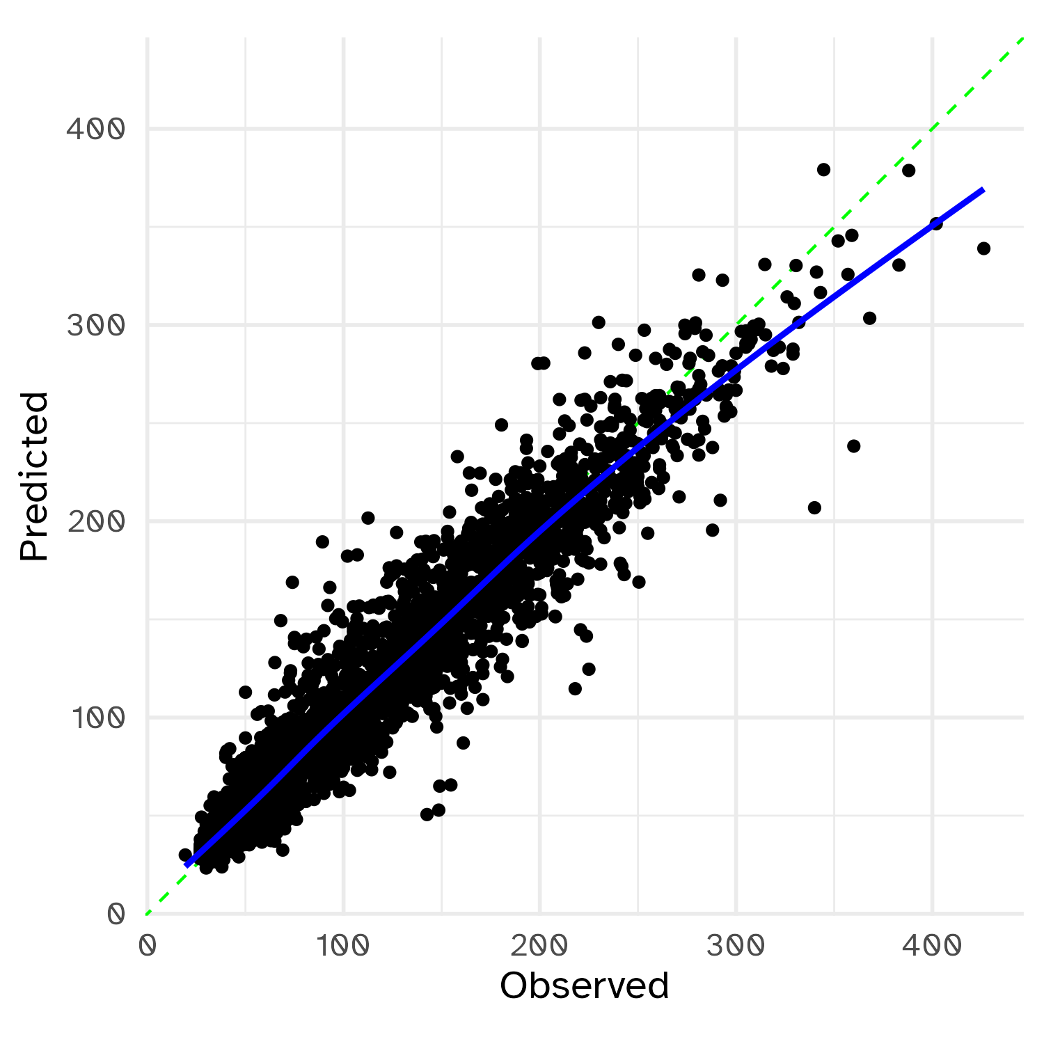
Checking calibration
Make your operations more efficient
Running in parallel
Grid search, combined with resampling, requires fitting a lot of models!
These models don’t depend on one another and can be run in parallel.
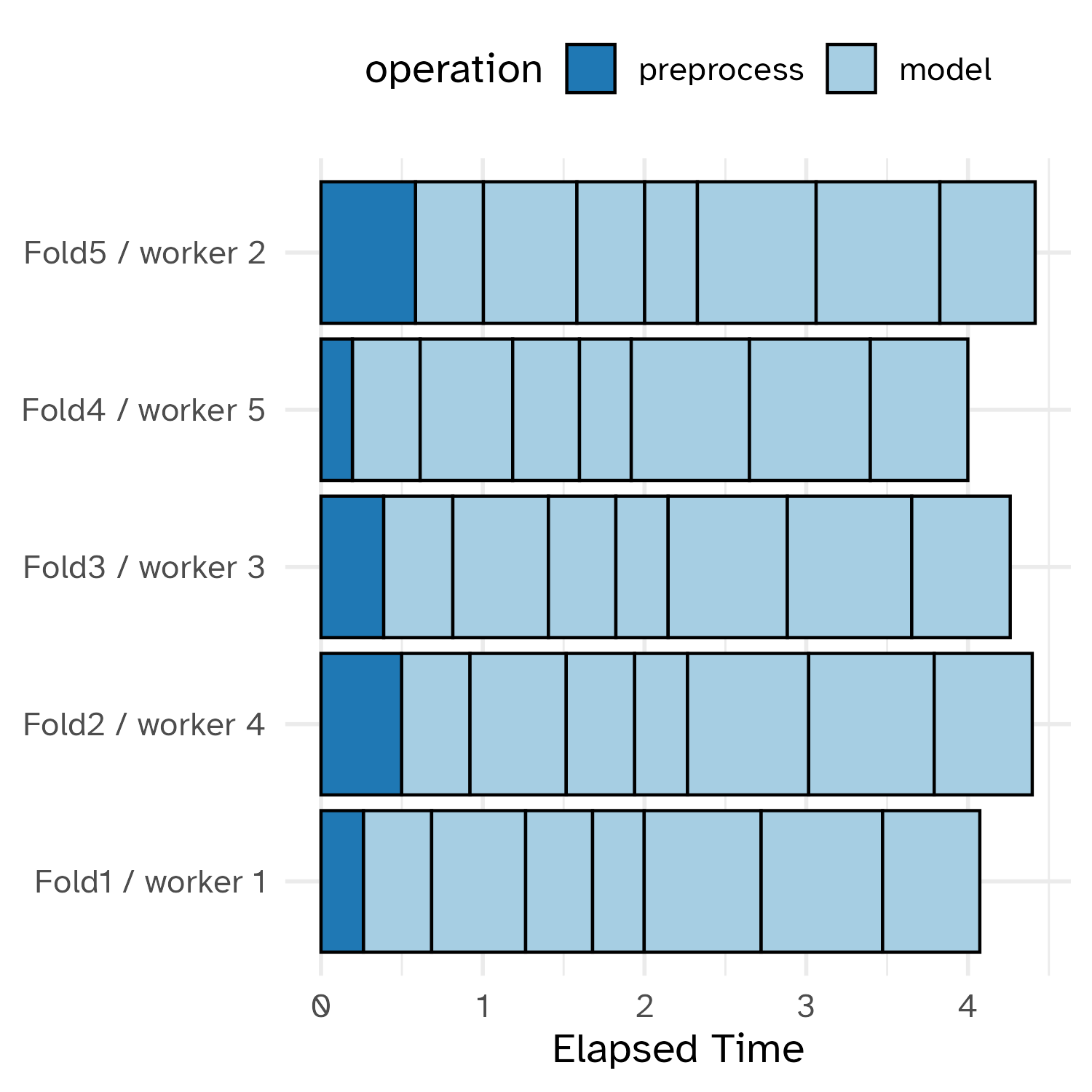
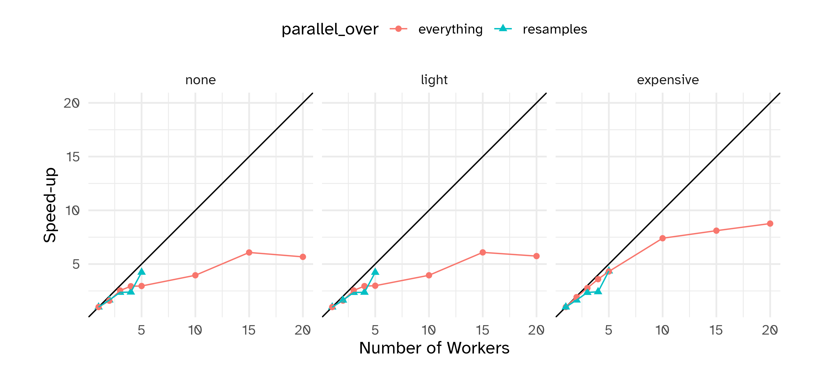
Running in parallel
Speed-ups are fairly linear up to the number of physical cores (10 here).
Early stopping for boosted trees
We have directly optimized the number of trees as a tuning parameter.
Instead we could
- Set the number of trees to a single large number.
- Stop adding trees when performance gets worse.
This is known as “early stopping” and there is a parameter for that: stop_iter.
Early stopping has a potential to decrease the tuning time.
Early stopping
lgbm_spec <- boost_tree(
  trees = 2000,
  learn_rate = tune(),
  stop_iter = tune(),
  min_n = tune()
) |>
  set_mode("regression") |>
  set_engine("lightgbm")

lgbm_wflow <- workflow(basic_rec, lgbm_spec)

# tune the model
lgbm_res <- lgbm_wflow |>
  tune_grid(
    resamples = hotel_rs,
    grid = 25,
    # The options below are not required by default
    control = ctrl,
    metrics = reg_metrics
  )
# A tibble: 5 × 9
  min_n learn_rate stop_iter .metric .estimator  mean     n std_err .config
  <int>      <dbl>     <int> <chr>   <chr>      <dbl> <int>   <dbl> <chr>
1     8    0.0422          8 mae     standard    11.7    10   0.242 Preprocessor1_Model05
2    21    0.0178          5 mae     standard    11.7    10   0.221 Preprocessor1_Model13
3    14    0.00750        17 mae     standard    11.9    10   0.222 Preprocessor1_Model09
4    25    0.1            10 mae     standard    12.2    10   0.217 Preprocessor1_Model16
5    35    0.00316         5 mae     standard    12.8    10   0.247 Preprocessor1_Model22
Our boosting model
Tree-based models (and a few others) don’t require indicators for categorical predictors. They can split on these variables as-is.
We’ll keep all categorical predictors as factors and focus on optimizing additional boosting parameters.
Our boosting model
lgbm_spec <- boost_tree(
  trees = 1000,
  learn_rate = tune(),
  min_n = tune(),
  tree_depth = tune(),
  loss_reduction = tune(),
  stop_iter = tune()
) |>
  set_mode("regression") |>
  set_engine("lightgbm")

lgbm_wflow <- workflow(avg_price_per_room ~ ., lgbm_spec)

lgbm_param <- lgbm_wflow |>
  extract_parameter_set_dials() |>
  update(learn_rate = learn_rate(c(-5, -1)))
Reduce your search space for tuning parameters where possible
Iterative search
Iterative search
Instead of pre-defining a grid of candidate points, we can model our current results to predict what the next candidate point should be.
Suppose that we are only tuning the learning rate in our boosted tree.
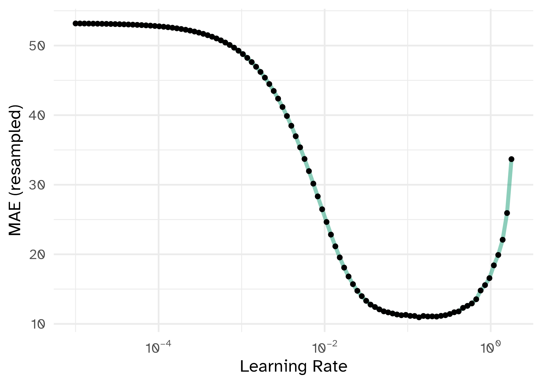
Iterative search
To illustrate the process, we resampled a large grid of learning rate values for our data to show what the relationship is between MAE and learning rate.
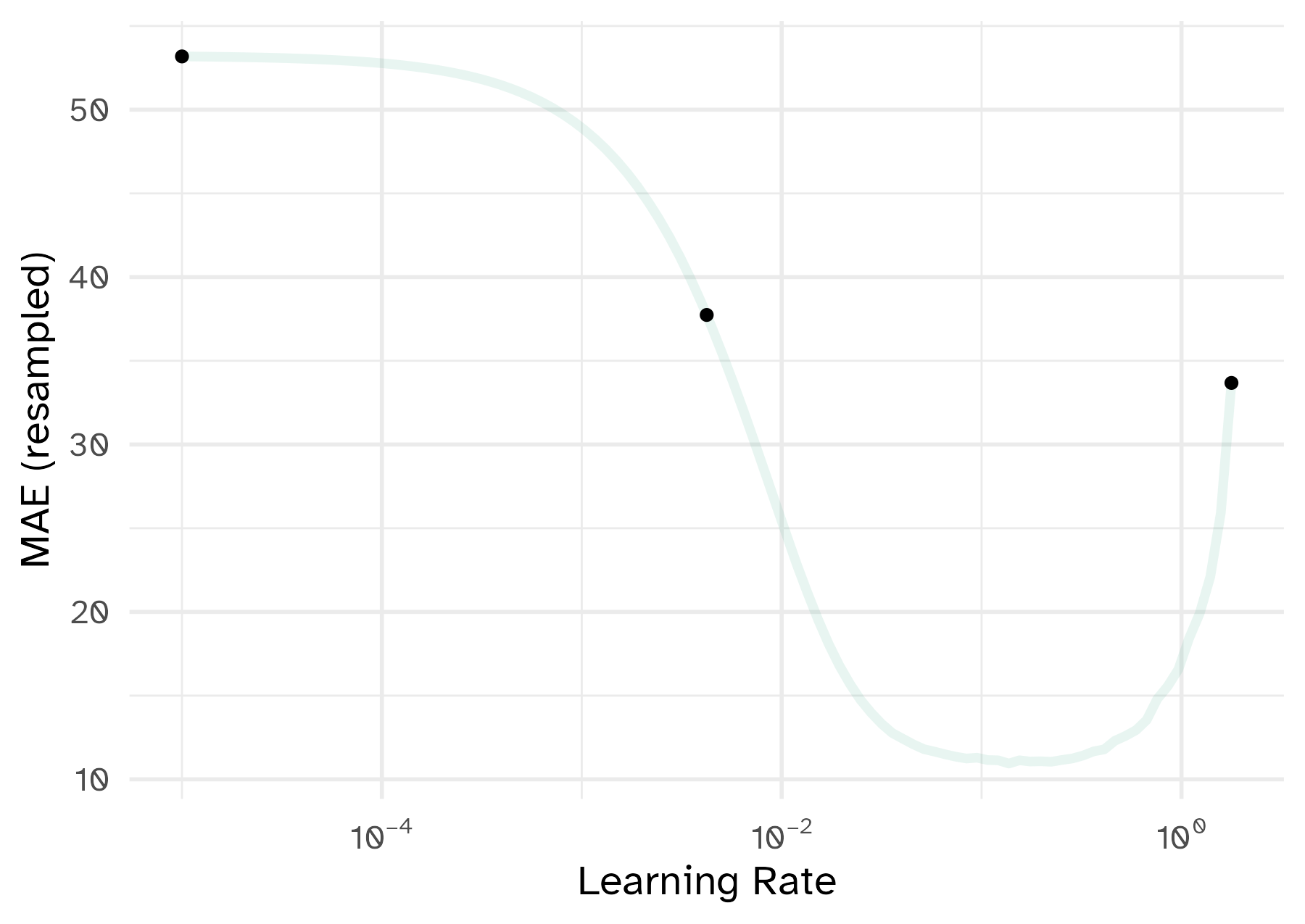
Now suppose that we used a grid of three points in the parameter range for learning rate…
A large grid
A three point grid
Bayesian optimization
- A sequential method that uses a model to predict new candidate parameters for assessment
- When scoring potential parameter value, the mean and variance of performance are predicted
- The strategy used to define how these two statistical quantities are used is defined by an acquisition function
Acquisition function
Acquisition functions take the predicted mean and variance and use them to balance:
- exploration: new candidates should explore new areas.
- exploitation: new candidates must stay near existing values.
Exploration focuses on the variance, exploitation is about the mean.
Iteratively search the parameter space using this approach to find an optimized set of candidate parameters.
Stop once a pre-defined number of iterations is reached or if no improvement is seen after a certain number of attempts.
Iteration evolution
Tuning using Bayesian optimization
Start with an initial set of candidate tuning parameter combinations and their performance estimates (e.g. grid search)
Rule of thumb: \(\text{number of initial points} = \text{number of tuning parameters} + 2\)
Initiate the iterative search process from this grid
scikit-learndoes not include Bayesian optimization functionality. Check outscikit-optimize.- It does include other iterative search methods like
RandomizedSearchCVand successive halving methodsHalvingGridSearchCVandHalvingRandomSearchCV.
An initial grid
# A tibble: 7 × 9
  min_n tree_depth learn_rate loss_reduction stop_iter  mean     n std_err .config
  <int>      <int>      <dbl>          <dbl>     <int> <dbl> <int>   <dbl> <chr>
1    33         12  0.0215          8.25e- 9         5  10.4    10   0.141 Preprocessor1_Model6
2    14         10  0.1             3.16e+ 1         8  10.6    10   0.184 Preprocessor1_Model3
3     8          3  0.00464         1   e-10        11  15.6    10   0.208 Preprocessor1_Model2
4    40          1  0.001           4.64e- 3        14  43.2    10   0.202 Preprocessor1_Model7
5    27         15  0.000215        6.81e- 7        20  44.7    10   0.238 Preprocessor1_Model5
6     2          5  0.0000464       3.83e- 1        17  51.2    10   0.283 Preprocessor1_Model1
7    21          8  0.00001         5.62e- 5         3  52.7    10   0.301 Preprocessor1_Model4
BO using {tidymodels}
Optimizing mae using the expected improvement── Iteration 1 ─────────────────────────────────────────────────────────────────────────────────────i Current best: mae=10.42 (@iter 0)i Gaussian process modeli Generating 5000 candidatesi Predicted candidatesi min_n=5, tree_depth=6, learn_rate=0.0976, loss_reduction=8.61e-10, stop_iter=7♥ Newest results: mae=10.02 (+/-0.127)── Iteration 2 ─────────────────────────────────────────────────────────────────────────────────────i Current best: mae=10.02 (@iter 1)i Gaussian process modeli Generating 5000 candidatesi Predicted candidatesi min_n=2, tree_depth=14, learn_rate=0.0204, loss_reduction=0.00276, stop_iter=9ⓧ Newest results: mae=10.07 (+/-0.18)── Iteration 3 ─────────────────────────────────────────────────────────────────────────────────────i Current best: mae=10.02 (@iter 1)i Gaussian process modeli Generating 5000 candidatesi Predicted candidatesi min_n=2, tree_depth=2, learn_rate=0.0125, loss_reduction=1.5e-06, stop_iter=11ⓧ Newest results: mae=13.85 (+/-0.241)── Iteration 4 ─────────────────────────────────────────────────────────────────────────────────────i Current best: mae=10.02 (@iter 1)i Gaussian process modeli Generating 5000 candidatesi Predicted candidatesi min_n=4, tree_depth=7, learn_rate=0.0493, loss_reduction=0.385, stop_iter=17♥ Newest results: mae=9.961 (+/-0.188)── Iteration 5 ─────────────────────────────────────────────────────────────────────────────────────i Current best: mae=9.961 (@iter 4)i Gaussian process modeli Generating 5000 candidatesi Predicted candidatesi min_n=38, tree_depth=1, learn_rate=0.0765, loss_reduction=3.46e-08, stop_iter=17ⓧ Newest results: mae=15.44 (+/-0.17)── Iteration 6 ─────────────────────────────────────────────────────────────────────────────────────i Current best: mae=9.961 (@iter 4)i Gaussian process modeli Generating 5000 candidatesi Predicted candidatesi min_n=5, tree_depth=13, learn_rate=0.0288, loss_reduction=2.58e-10, stop_iter=6ⓧ Newest results: mae=10.04 (+/-0.184)── Iteration 7 ─────────────────────────────────────────────────────────────────────────────────────i Current best: mae=9.961 (@iter 4)i Gaussian process modeli Generating 5000 candidatesi Predicted candidatesi min_n=18, tree_depth=15, learn_rate=0.0117, loss_reduction=1.72, stop_iter=15ⓧ Newest results: mae=10.68 (+/-0.197)── Iteration 8 ─────────────────────────────────────────────────────────────────────────────────────i Current best: mae=9.961 (@iter 4)i Gaussian process modeli Generating 5000 candidatesi Predicted candidatesi min_n=2, tree_depth=14, learn_rate=0.0747, loss_reduction=0.00194, stop_iter=12♥ Newest results: mae=9.784 (+/-0.175)── Iteration 9 ─────────────────────────────────────────────────────────────────────────────────────i Current best: mae=9.784 (@iter 8)i Gaussian process modeli Generating 5000 candidatesi Predicted candidatesi min_n=26, tree_depth=15, learn_rate=0.0429, loss_reduction=1.39, stop_iter=11ⓧ Newest results: mae=10.12 (+/-0.138)── Iteration 10 ────────────────────────────────────────────────────────────────────────────────────i Current best: mae=9.784 (@iter 8)i Gaussian process modeli Generating 5000 candidatesi Predicted candidatesi min_n=20, tree_depth=15, learn_rate=0.021, loss_reduction=1.76e-07, stop_iter=6ⓧ Newest results: mae=10.37 (+/-0.169)── Iteration 11 ────────────────────────────────────────────────────────────────────────────────────i Current best: mae=9.784 (@iter 8)i Gaussian process modeli Generating 5000 candidatesi Predicted candidatesi min_n=4, tree_depth=8, learn_rate=0.0656, loss_reduction=26.8, stop_iter=7ⓧ Newest results: mae=10.33 (+/-0.182)── Iteration 12 ────────────────────────────────────────────────────────────────────────────────────i Current best: mae=9.784 (@iter 8)i Gaussian process modeli Generating 5000 candidatesi Predicted candidatesi min_n=2, tree_depth=14, learn_rate=0.0541, loss_reduction=2.22e-06, stop_iter=17ⓧ Newest results: mae=9.93 (+/-0.184)── Iteration 13 ────────────────────────────────────────────────────────────────────────────────────i Current best: mae=9.784 (@iter 8)i Gaussian process modeli Generating 5000 candidatesi Predicted candidatesi min_n=4, tree_depth=7, learn_rate=0.00959, loss_reduction=12.8, stop_iter=3ⓧ Newest results: mae=10.63 (+/-0.213)── Iteration 14 ────────────────────────────────────────────────────────────────────────────────────i Current best: mae=9.784 (@iter 8)i Gaussian process modeli Generating 5000 candidatesi Predicted candidatesi min_n=4, tree_depth=15, learn_rate=0.095, loss_reduction=6.98e-08, stop_iter=8ⓧ Newest results: mae=9.88 (+/-0.157)── Iteration 15 ────────────────────────────────────────────────────────────────────────────────────i Current best: mae=9.784 (@iter 8)i Gaussian process modeli Generating 5000 candidatesi Predicted candidatesi min_n=2, tree_depth=14, learn_rate=0.00638, loss_reduction=0.00978, stop_iter=16ⓧ Newest results: mae=11.06 (+/-0.223)── Iteration 16 ────────────────────────────────────────────────────────────────────────────────────i Current best: mae=9.784 (@iter 8)i Gaussian process modeli Generating 5000 candidatesi Predicted candidatesi min_n=7, tree_depth=7, learn_rate=0.0339, loss_reduction=0.0822, stop_iter=17ⓧ Newest results: mae=9.975 (+/-0.165)── Iteration 17 ────────────────────────────────────────────────────────────────────────────────────i Current best: mae=9.784 (@iter 8)i Gaussian process modeli Generating 5000 candidatesi Predicted candidatesi min_n=5, tree_depth=14, learn_rate=0.0868, loss_reduction=0.00256, stop_iter=6ⓧ Newest results: mae=10 (+/-0.18)── Iteration 18 ────────────────────────────────────────────────────────────────────────────────────i Current best: mae=9.784 (@iter 8)i Gaussian process modeli Generating 5000 candidatesi Predicted candidatesi min_n=3, tree_depth=12, learn_rate=0.0391, loss_reduction=0.00133, stop_iter=13ⓧ Newest results: mae=9.914 (+/-0.174)! No improvement for 10 iterations; returning current results.Best results
# A tibble: 5 × 10
min_n tree_depth learn_rate loss_reduction stop_iter mean n std_err .config .iter
<int> <int> <dbl> <dbl> <int> <dbl> <int> <dbl> <chr> <int>
1 2 14 0.0747 0.00194 12 9.78 10 0.175 Iter8 8
2 4 15 0.0950 0.0000000698 8 9.88 10 0.157 Iter14 14
3 3 12 0.0391 0.00133 13 9.91 10 0.174 Iter18 18
4 2 14 0.0541 0.00000222 17 9.93 10 0.184 Iter12 12
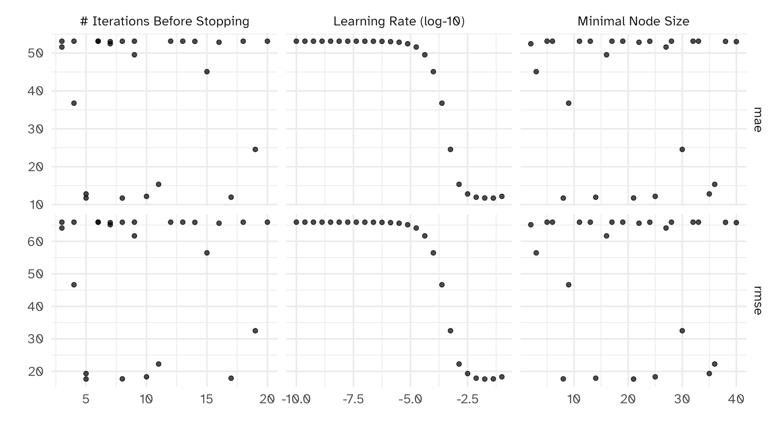
5 4 7 0.0493 0.385 17 9.96 10 0.188 Iter4 4Plotting BO results
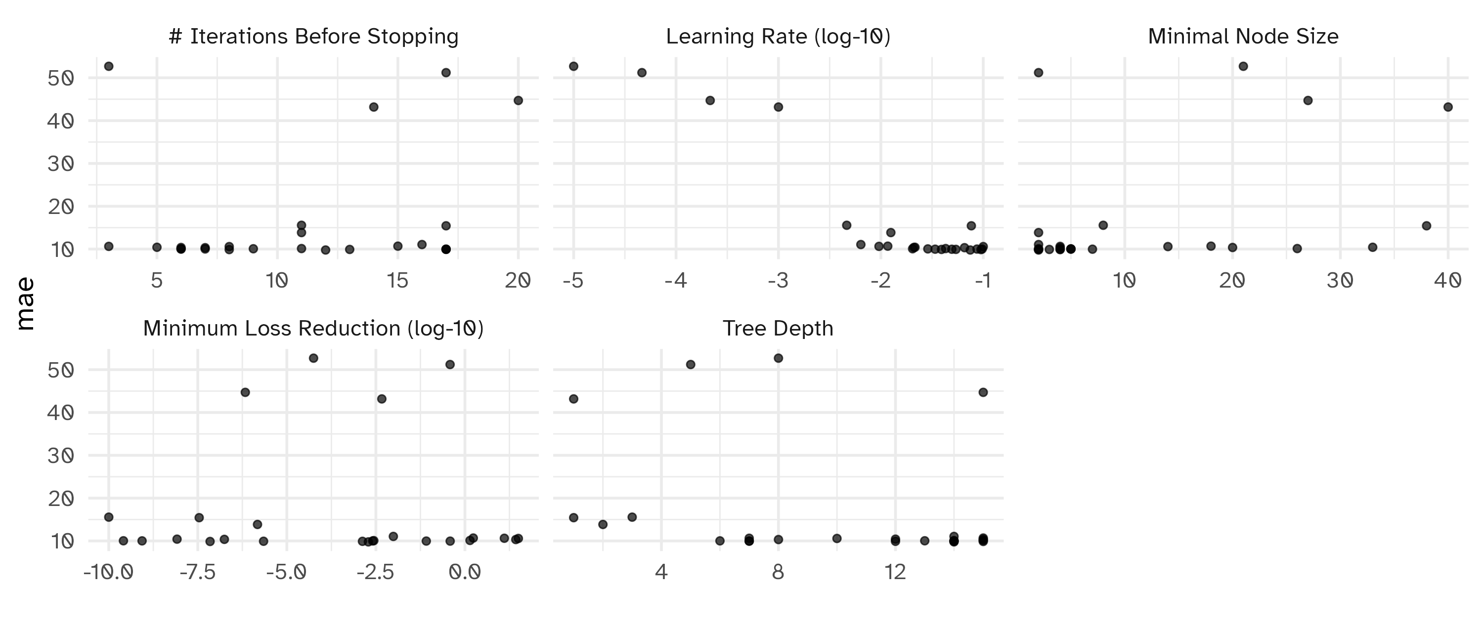
Notes on iterative search
Fewer benefits from parallel processing since the process is sequential.
Parallel processing can still be used to more efficiently measure each candidate point.
There are a lot of other iterative methods that you can use.
Finalizing the model
Finalizing the model
Let’s say that we’ve tried a lot of different models and we like our LightGBM model the most.
What do we do now?
- Finalize the workflow by choosing the values for the tuning parameters.
- Fit the model on the entire training set.
- Verify performance using the test set.
- Document and publish the model (later this semester)
Locking down the tuning parameters
We can take the results of the Bayesian optimization and accept the best results:
══ Workflow ════════════════════════════════════════════════════════════════════════════════════════
Preprocessor: Formula
Model: boost_tree()

── Preprocessor ────────────────────────────────────────────────────────────────────────────────────
avg_price_per_room ~ .

── Model ───────────────────────────────────────────────────────────────────────────────────────────
Boosted Tree Model Specification (regression)

Main Arguments:
  trees = 1000
  min_n = 2
  tree_depth = 14
  learn_rate = 0.074693488320648
  loss_reduction = 0.0019429235832599
  stop_iter = 12

Computational engine: lightgbm
The model with the best parameters can be extracted from the *SearchCV object from the best_estimator_ attribute. Use this to make predictions on new data.
The final fit
We can use individual functions:
# Resampling results
# Manual resampling
# A tibble: 1 × 6
  splits              id               .metrics         .notes           .predictions .workflow
  <list>              <chr>            <list>           <list>           <list>       <list>
1 <split [3749/1251]> train/test split <tibble [2 × 4]> <tibble [0 × 3]> <tibble>     <workflow>
Test set results
# A tibble: 2 × 4
  .metric .estimator .estimate .config
  <chr>   <chr>          <dbl> <chr>
1 rmse    standard       15.1  Preprocessor1_Model1
2 mae     standard        9.62 Preprocessor1_Model1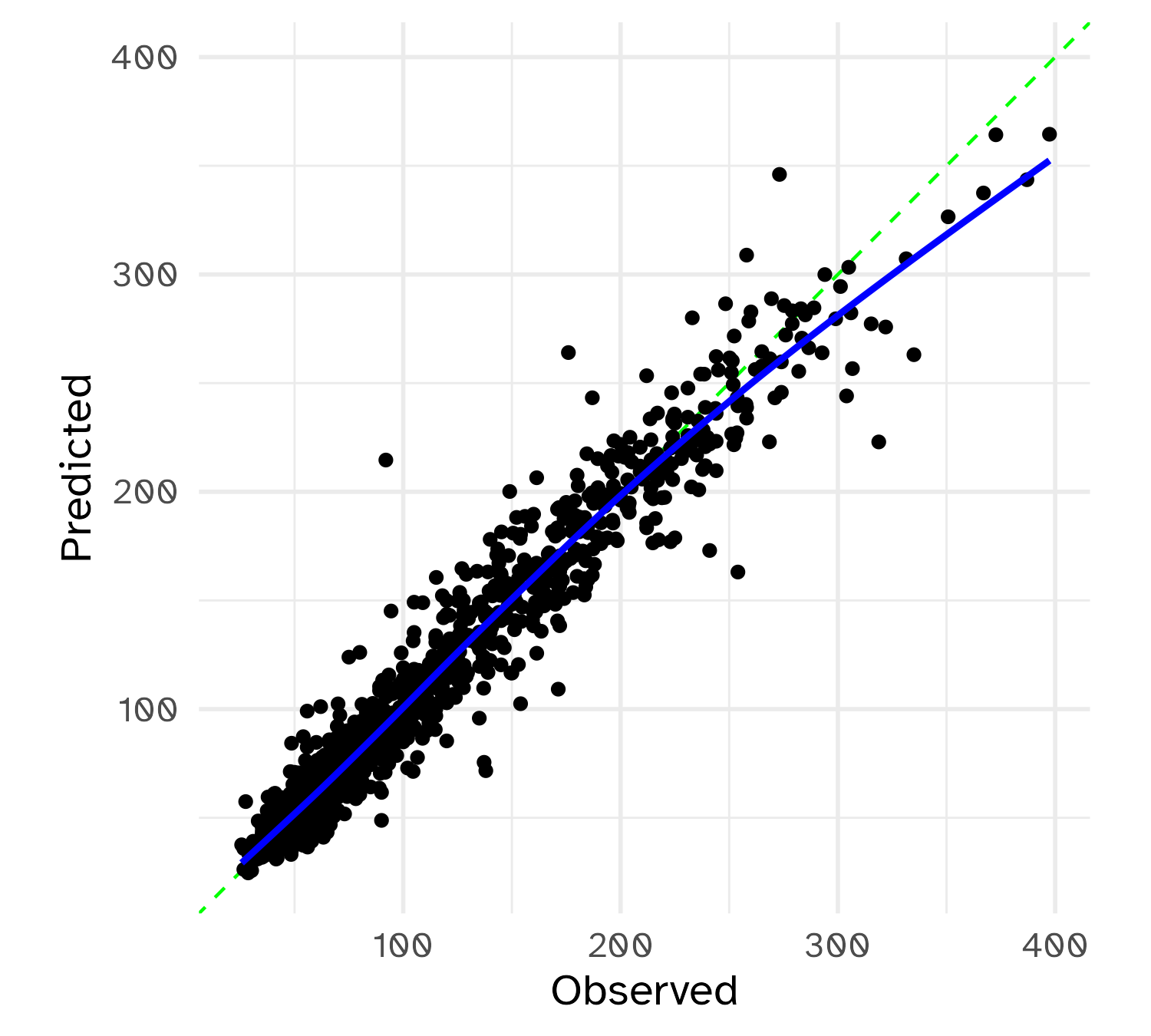
Recall that resampling predicted the MAE to be 9.78.
Wrap-up
Recap
- Tuning parameters significantly impact the performance of models
- Tuning parameters can be defined in both the feature engineering and model specification stages
- Grid search is a simple but effective method for tuning parameters
- Iterative search methods can be used to optimize parameters
- Bayesian optimization is a sequential method that uses a model to predict new candidate parameters for assessment
Acknowledgments
- Materials derived in part from Machine learning with {tidymodels} and licensed under a Creative Commons Attribution-ShareAlike 4.0 International (CC BY-SA) License.