# A tibble: 7,107 × 20
   forested  year elevation eastness northness roughness tree_no_tree dew_temp precip_annual
   <fct>    <dbl>     <dbl>    <dbl>     <dbl>     <dbl> <fct>           <dbl>         <dbl>
 1 Yes       2005       881       90        43        63 Tree             0.04           466
 2 Yes       2005       113      -25        96        30 Tree             6.4           1710
 3 No        2005       164      -84        53        13 Tree             6.06          1297
 4 Yes       2005       299       93        34         6 No tree          4.43          2545
 5 Yes       2005       806       47       -88        35 Tree             1.06           609
 6 Yes       2005       736      -27       -96        53 Tree             1.35           539
 7 Yes       2005       636      -48        87         3 No tree          1.42           702
 8 Yes       2005       224      -65       -75         9 Tree             6.39          1195
 9 Yes       2005        52      -62        78        42 Tree             6.5           1312
10 Yes       2005      2240      -67       -74        99 No tree         -5.63          1036
# ℹ 7,097 more rows
# ℹ 11 more variables: temp_annual_mean <dbl>, temp_annual_min <dbl>, temp_annual_max <dbl>,
#   temp_january_min <dbl>, vapor_min <dbl>, vapor_max <dbl>, canopy_cover <dbl>, lon <dbl>,
# lat <dbl>, land_type <fct>, county <fct>Evaluate models using appropriate metrics
Lecture 8
September 18, 2025
Data on forests in Washington
- The U.S. Forest Service maintains ML models to predict whether a plot of land is “forested.”
- This classification is important for all sorts of research, legislation, and land management purposes.
- Plots are typically remeasured every 10 years and this dataset contains the most recent measurement per plot.

Data on forests in Washington
N = 7,107plots of land, one from each of 7,107 6000-acre hexagons in WA.- A nominal outcome,
forested, with levels"Yes"and"No", measured “on-the-ground.” - 18 remotely-sensed and easily-accessible predictors:
- numeric variables based on weather and topography.
- nominal variables based on classifications from other governmental orgs.

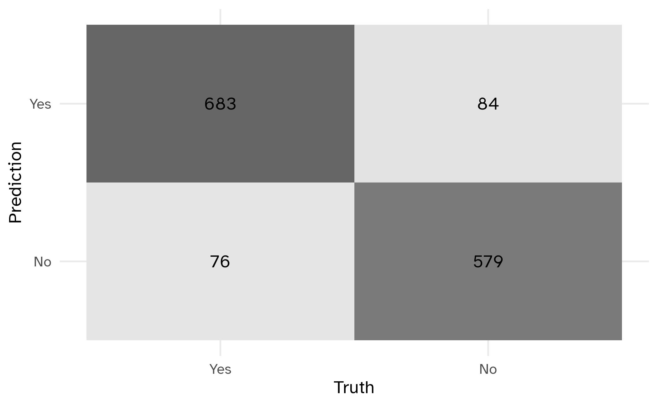
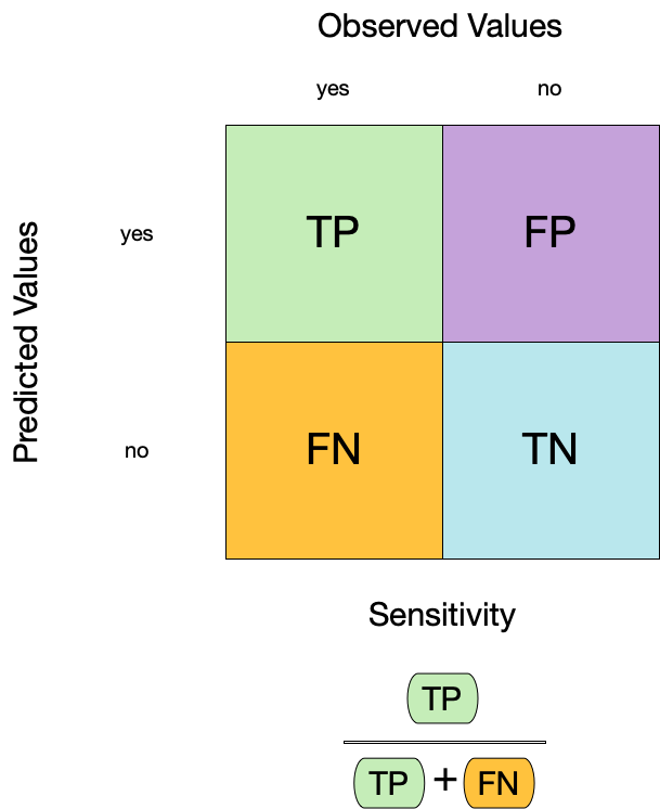
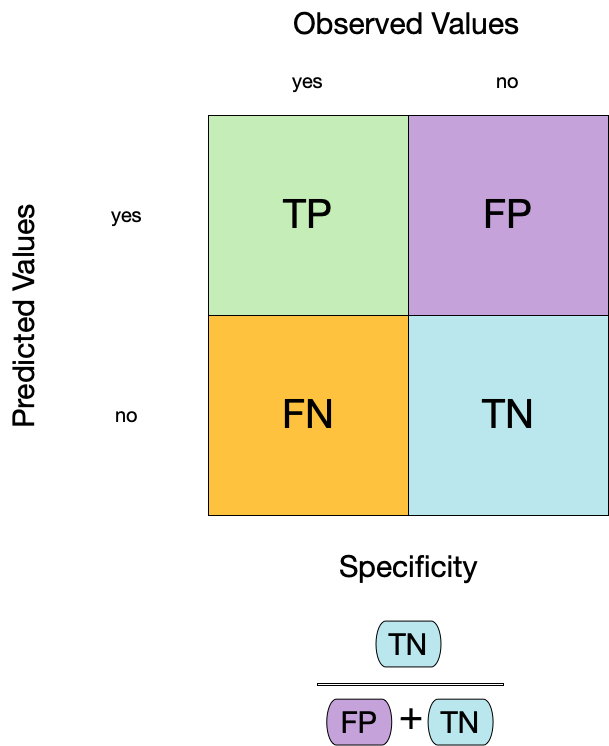
Confusion matrix
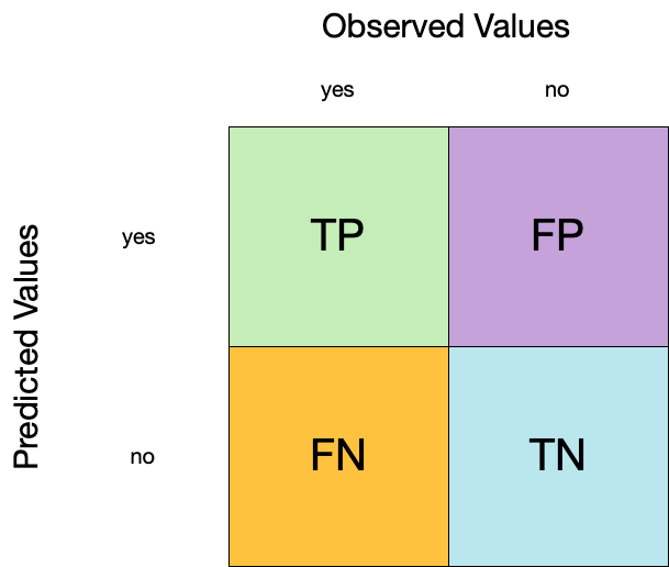
Confusion matrix
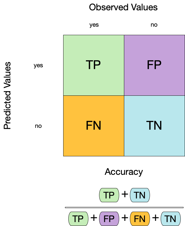
Metrics for model performance
Sensitivity (TPR)
Specificity (TNR)
📝 Group differences in metrics
# A tibble: 6 × 4
  tree_no_tree .metric     .estimator .estimate
  <fct>        <chr>       <chr>          <dbl>
1 Tree         accuracy    binary         0.899
2 No tree      accuracy    binary         0.876
3 Tree         specificity binary         0.372
4 No tree      specificity binary         0.940
5 Tree         sensitivity binary         0.964
6 No tree      sensitivity binary         0.583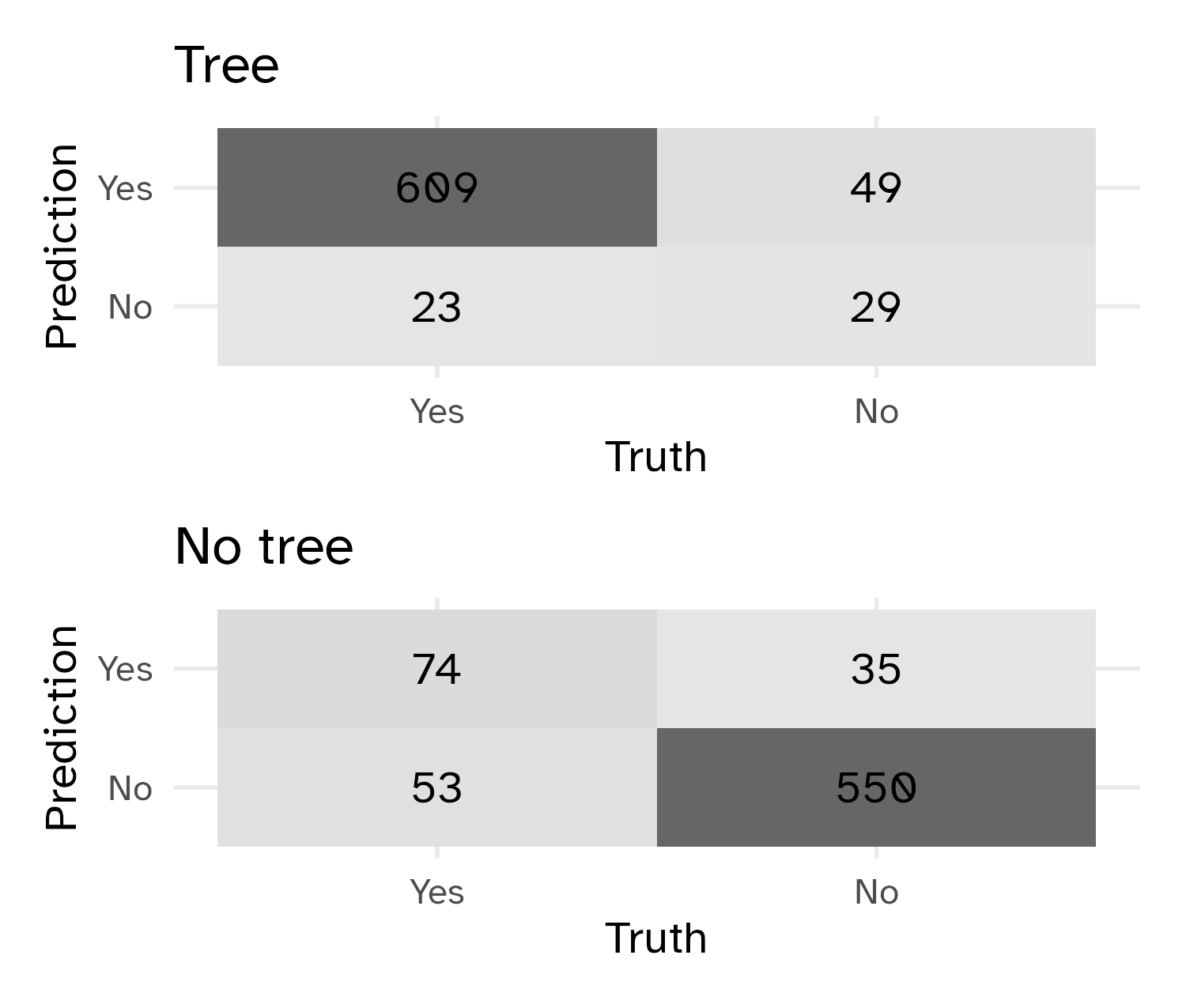
03:00
Varying the threshold
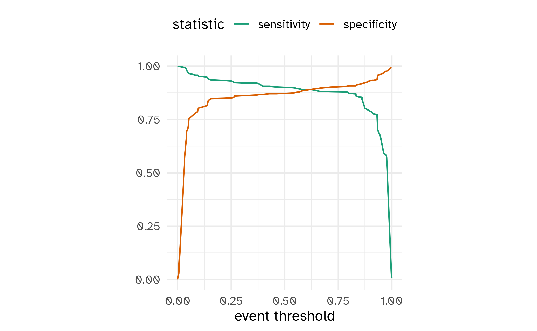
ROC curves
For an ROC (receiver operator characteristic) curve, we plot
- the false positive rate (1 - specificity) on the x-axis
- the true positive rate (sensitivity) on the y-axis
with sensitivity and specificity calculated at all possible thresholds.
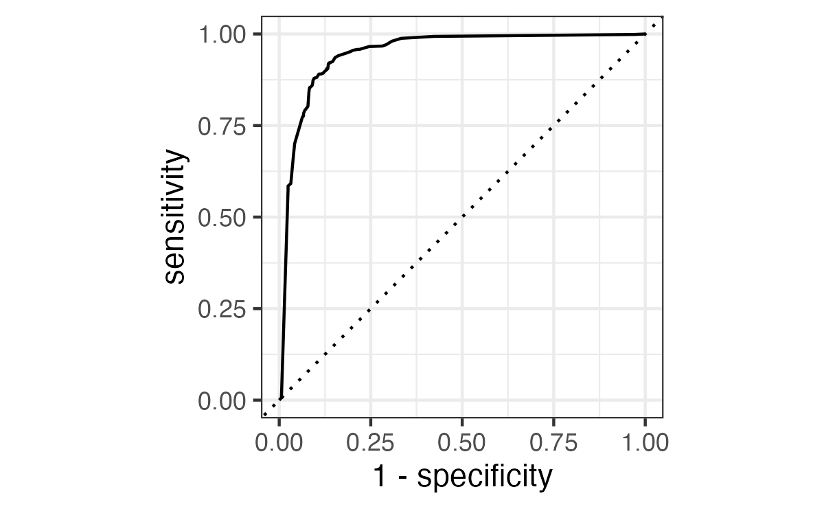
ROC curves
We can use the area under the ROC curve as a classification metric:
- ROC AUC = 1 💯
- ROC AUC = 1/2 😢

ROC curves
Show the code

# A tibble: 1 × 3
  .metric .estimator .estimate
  <chr>   <chr>          <dbl>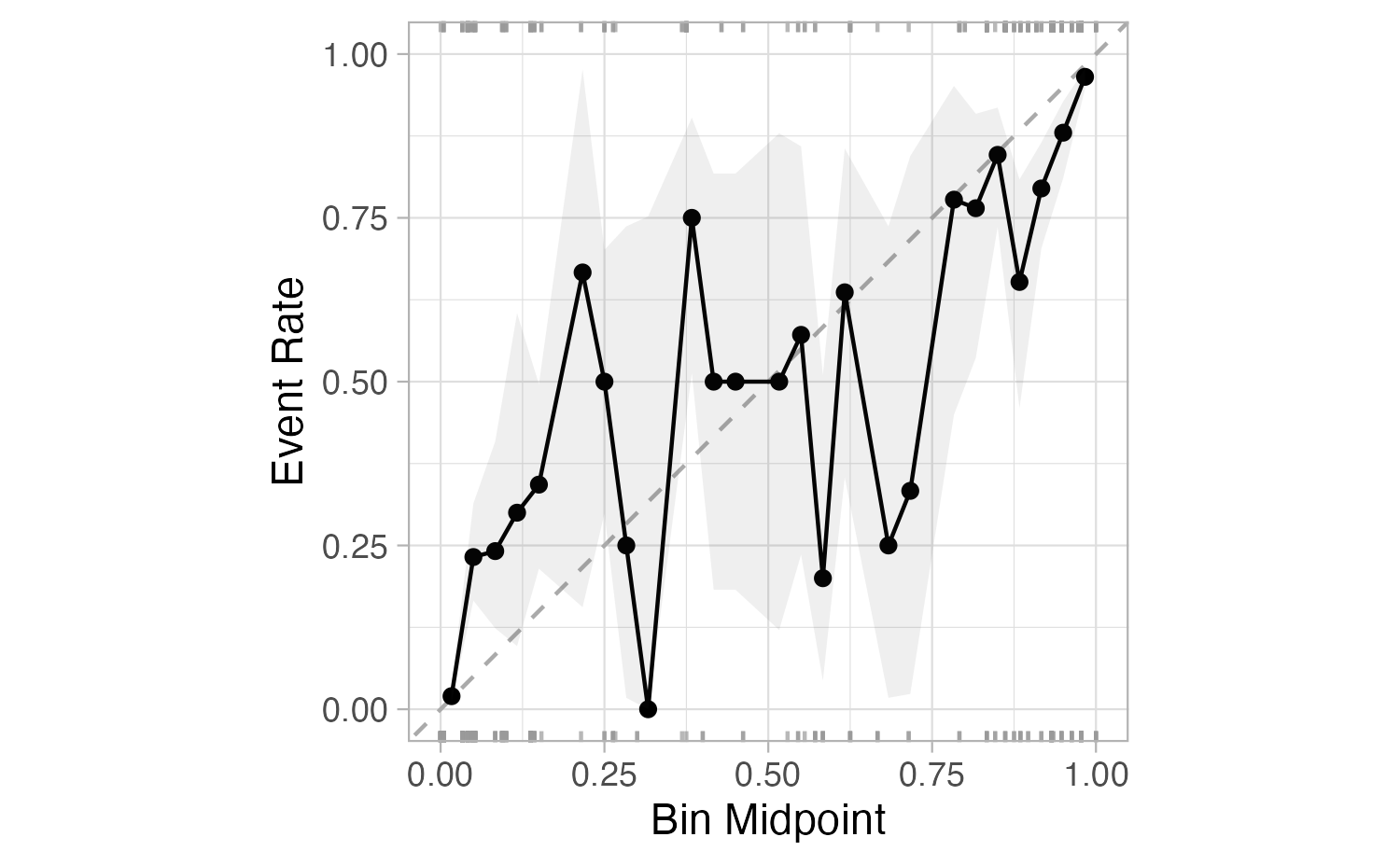
1 roc_auc binary 0.948Separation vs calibration
The ROC captures separation
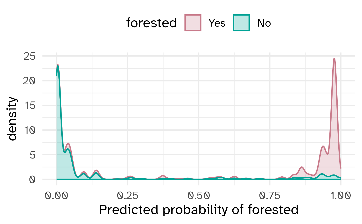
The Brier score captures calibration