Explaining models through agnostic approaches
Lecture 13
Dr. Benjamin Soltoff
Cornell University
INFO 4940/5940 - Fall 2025
October 7, 2025
Announcements
Announcements
- Homework 4 due tomorrow
- Project proposals due Thursday
- No class Thursday
- Dr. Soltoff’s office hours cancelled tomorrow
Learning objectives
- Review the importance of explainability for machine learning models
- Identify techniques for local and global explanations of machine learning predictions
- Implement Shapley values for local explanations
- Estimate permutation-based feature importance measures
- Evaluate marginal effects of features using partial dependence plots
Explainability
Explanation
Answer to the “why” question
- Why was my mortgage application denied?
- Why does Zillow think my house is worth $250,000?
- Why did Netflix recommend K-Pop: Demon Hunters?
What is a good explanation?
- Contrastive: why was this prediction made instead of another prediction?
- Selected: Focuses on just a handful of reasons, even if the problem is more complex
- Social: Needs to be understandable by your audience
- Truthful: Explanation should predict the event as truthfully as possible
- Generalizable: Explanation could apply to many predictions
Types of model explanations
White-box model
Models that lend themselves naturally to interpretation
- Linear regression
- Logistic regression
- Generalized linear model
- Decision tree

Image credit: xkcd
Black-box model
- Random forests
- Boosted trees
- Neural networks
- Deep learning
Predicting student debt
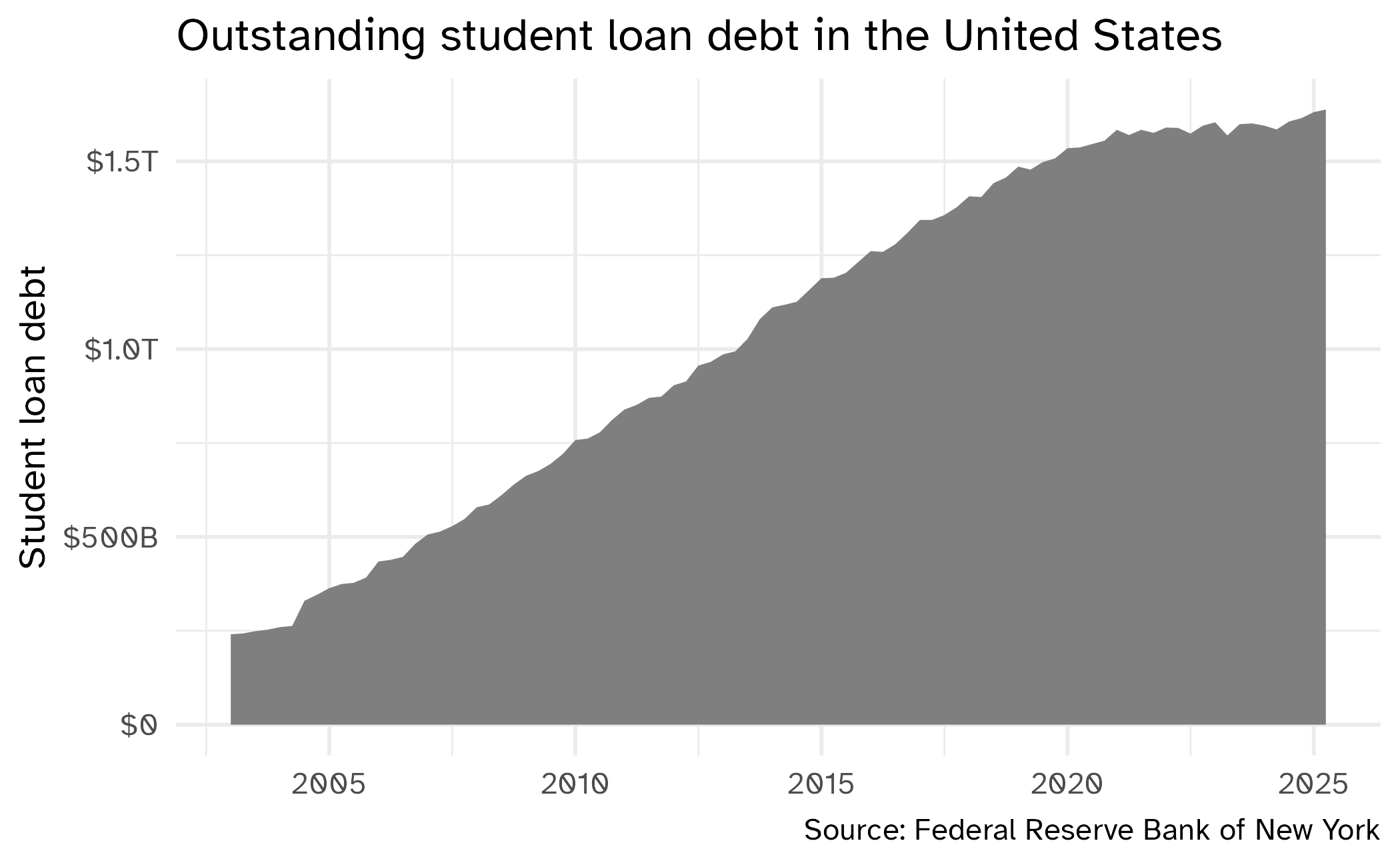
Data source: Federal Reserve Bank of New York
Predicting student debt
Rows: 2,659
Columns: 28
$ unit_id             <dbl> 100654, 100663, 100690, 100706, 100724, 100751, 100812, 100830, 100858…
$ name                <chr> "Alabama A & M University", "University of Alabama at Birmingham", "Am…
$ state               <chr> "AL", "AL", "AL", "AL", "AL", "AL", "AL", "AL", "AL", "AL", "AL", "AL"…
$ act_med             <dbl> 18, 27, NA, 28, 18, 26, NA, 21, NA, 25, NA, 20, NA, 22, NA, 20, 19, NA…
$ adm_rate            <dbl> 0.6622, 0.8842, NA, 0.7425, 0.9564, 0.7582, NA, 0.9263, 0.5047, 0.5194…
$ comp_rate           <dbl> 0.2874, 0.6260, 0.4000, 0.6191, 0.3018, 0.7369, NA, 0.3568, 0.7921, 0.…
$ cost_net            <dbl> 14559, 17727, NA, 19880, 13889, 22150, NA, 14596, 23897, 23351, 25157,…
$ cost_sticker        <dbl> 23751, 27826, NA, 27098, 22028, 32024, NA, 21873, 34402, 38385, 30704,…
$ death_pct           <dbl> NA, NA, NA, NA, NA, NA, NA, NA, NA, NA, 0.003513514, NA, 0.003789793, …
$ debt                <dbl> 16600, 15832, 13385, 13905, 17500, 17986, 14861, 13119, 17750, 16000, …
$ earnings_med        <dbl> 27851, 46572, 30377, 55610, 27453, 52233, 46266, 38216, 54629, 45229, …
$ earnings_sd         <dbl> 25637, 42095, 24493, 36093, 37402, 59300, 32307, 28205, 46748, NA, 352…
$ faculty_full_time   <dbl> 0.7146, 0.7584, 1.0000, 0.6308, 0.6637, 0.7836, 0.4783, 0.6955, 0.8587…
$ faculty_salary_mean <dbl> 77490, 109899, 45981, 93699, 72135, 99810, 85068, 79407, 107163, 59274…
$ female              <dbl> 0.5640301, 0.6390907, 0.6486486, 0.4763499, 0.6134185, 0.6152524, 0.70…
$ first_gen           <dbl> 0.3658281, 0.3412237, 0.5125000, 0.3101322, 0.3434343, 0.2257127, 0.47…
$ instruct_exp        <dbl> 6298, 17179, 5671, 9461, 11082, 9380, 9639, 7006, 10041, 10898, 7449, …
$ locale              <chr> "City", "City", "City", "City", "City", "City", "Town", "City", "City"…
$ median_hh_inc       <dbl> 49720, 55735, 53683, 58688, 46065, 57928, 50752, 50723, 59005, 64789, …
$ open_admissions     <chr> "No", "No", "Yes", "No", "No", "No", NA, "No", "No", "No", "Yes", "No"…
$ pbi                 <chr> "No", "No", "No", "No", "No", "No", "No", "Yes", "No", "No", "No", "Ye…
$ pell_pct            <dbl> 0.6441, 0.3318, 0.6842, 0.2250, 0.7203, 0.1799, 0.4238, 0.4275, 0.1226…
$ retention_rate      <dbl> 0.6387, 0.8195, NA, 0.8050, 0.6045, 0.8609, NA, 0.6580, 0.9319, 0.6311…
$ sat_mean            <dbl> 947, 1251, NA, 1321, 977, 1287, NA, 1090, 1318, 1197, NA, 1016, NA, 11…
$ test_policy         <chr> "Considered but not required", "Considered but not required", NA, "Con…
$ type                <chr> "Public", "Public", "Private, nonprofit", "Public", "Public", "Public"…
$ veteran             <dbl> 0.003138732, 0.003167505, 0.040540540, NA, NA, 0.003974221, NA, 0.0048…
$ women_only          <chr> "No", "No", "No", "No", "No", "No", "No", "No", "No", "No", "No", "No"…
Fitted models
library(tidyverse)
library(tidymodels)
library(here)
# get scorecard dataset
scorecard <- read_csv(file = here("slides/data/scorecard.csv")) |>
# remove ID columns - causing issues when interpreting/explaining
select(-unit_id, -name) |>
# convert factor to character columns
mutate(across(.cols = where(is.factor), .f = as.character))
# split into training and testing
set.seed(123)
scorecard_split <- initial_split(data = scorecard, prop = .75, strata = debt)
scorecard_train <- training(scorecard_split)
scorecard_test <- testing(scorecard_split)
scorecard_folds <- vfold_cv(data = scorecard_train, v = 10)
# basic feature engineering recipe
scorecard_rec <- recipe(debt ~ ., data = scorecard_train) |>
# catch all category for missing state values
step_novel(state) |>
# use median imputation for numeric predictors
step_impute_median(all_numeric_predictors()) |>
# use modal imputation for nominal predictors
step_impute_mode(all_nominal_predictors()) |>
# remove rows with missing values for
# outcomes - glmnet won't work if any of this column is NA
step_naomit(all_outcomes())
# generate random forest model
rf_mod <- rand_forest() |>
set_engine("ranger") |>
set_mode("regression")
# combine recipe with model
rf_wf <- workflow() |>
add_recipe(scorecard_rec) |>
add_model(rf_mod)
# fit using training set
set.seed(123)
rf_wf <- fit(
rf_wf,
data = scorecard_train
)
# fit penalized regression model
## recipe
glmnet_recipe <- scorecard_rec |>
# use median imputation for numeric predictors
step_impute_median(all_numeric_predictors()) |>
step_dummy(all_nominal_predictors()) |>
step_zv(all_predictors()) |>
step_normalize(all_numeric_predictors())
## model specification
glmnet_spec <- linear_reg(penalty = tune(), mixture = tune()) |>
set_mode("regression") |>
set_engine("glmnet")
## workflow
glmnet_workflow <- workflow() |>
add_recipe(glmnet_recipe) |>
add_model(glmnet_spec)
## tuning grid
glmnet_grid <- expand_grid(
penalty = 10^seq(-6, -1, length.out = 20),
mixture = c(0.05, 0.2, 0.4, 0.6, 0.8, 1)
)
## hyperparameter tuning
glmnet_tune <- tune_grid(
glmnet_workflow,
resamples = scorecard_folds,
grid = glmnet_grid
)
# select best model
glmnet_best <- select_best(glmnet_tune, metric = "rmse")
glmnet_wf <- finalize_workflow(glmnet_workflow, glmnet_best) |>
last_fit(scorecard_split) |>
extract_workflow()
# nearest neighbors model
## use glmnet recipe
kknn_spec <- nearest_neighbor(neighbors = 10) |>
set_mode("regression") |>
set_engine("kknn")
kknn_workflow <-
workflow() |>
add_recipe(glmnet_recipe) |>
add_model(kknn_spec)
## fit using training set
set.seed(123)
kknn_wf <- fit(
kknn_workflow,
data = scorecard_train
)
# save all required objects to a .Rdata file
save(
scorecard_train,
scorecard_test,
rf_wf,
glmnet_wf,
kknn_wf,
file = here("slides/data/scorecard-models.RData")
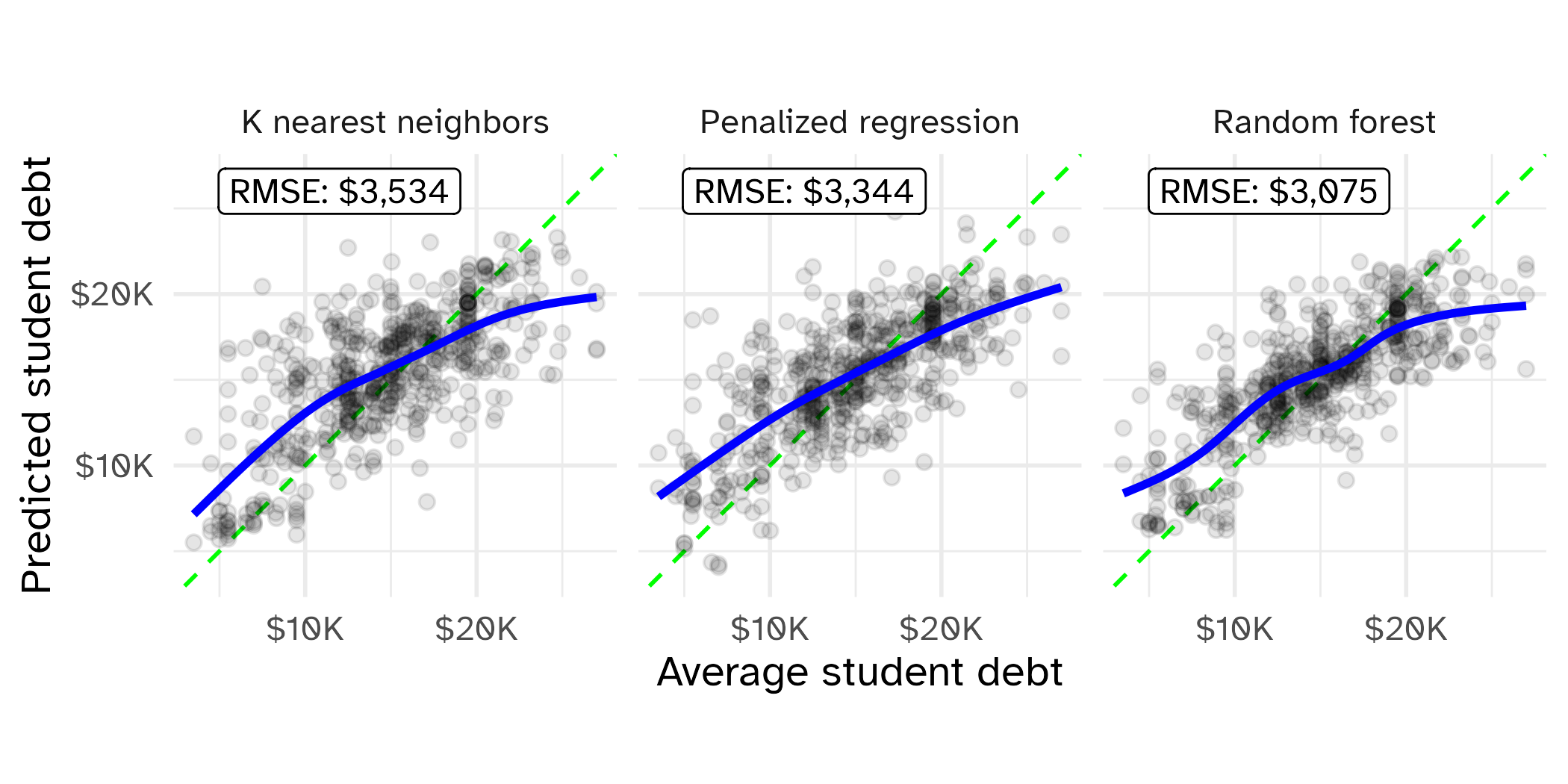
)Evaluating test set performance
Explainers with {DALEX}
{DALEX}
Framework for explainable AI in R and Python
- Model-agnostic approach to explainability
- Local and global explanations
- Works with any machine learning model
- Integrates with {tidymodels} and
scikit-learn
More info: DALEX documentation
Create an explainer object
explainer_glmnet <- explain_tidymodels(
  model = glmnet_wf,
  data = scorecard_train |> select(-debt),
  y = scorecard_train$debt,
  label = "penalized regression",
  verbose = FALSE
)

explainer_rf <- explain_tidymodels(
  model = rf_wf,
  data = scorecard_train |> select(-debt),
  y = scorecard_train$debt,
  label = "random forest",
  verbose = FALSE
)

explainer_kknn <- explain_tidymodels(
  model = kknn_wf,
  data = scorecard_train |> select(-debt),
  y = scorecard_train$debt,
  label = "k nearest neighbors",
  verbose = FALSE
)
See the Explainer class.
Local explanations
Local explanations
Provide information about a prediction for a single observation.
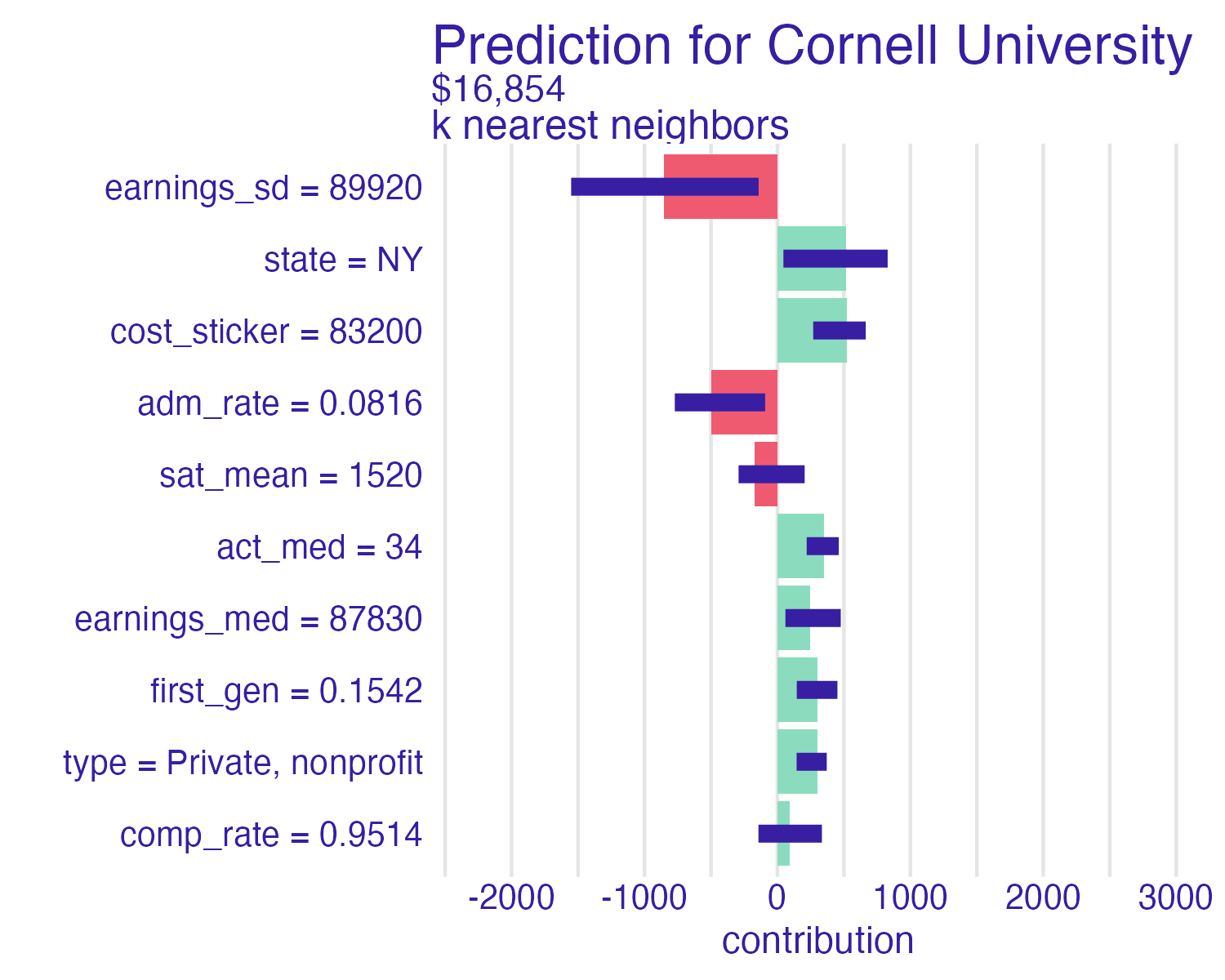
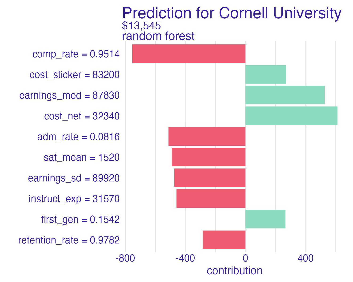
Cornell University
Rows: 1
Columns: 26
$ state <chr> "NY"
$ act_med <dbl> 34
$ adm_rate <dbl> 0.0816
$ comp_rate <dbl> 0.9514
$ cost_net <dbl> 32337
$ cost_sticker <dbl> 83196
$ death_pct <dbl> NA
$ debt <dbl> 13000
$ earnings_med <dbl> 87830
$ earnings_sd <dbl> 89915
$ faculty_full_time <dbl> 0.9233
$ faculty_salary_mean <dbl> 155277
$ female <dbl> 0.5335581
$ first_gen <dbl> 0.154164
$ instruct_exp <dbl> 31572
$ locale <chr> "City"
$ median_hh_inc <dbl> 80346
$ open_admissions <chr> "No"
$ pbi <chr> "No"
$ pell_pct <dbl> 0.1821
$ retention_rate <dbl> 0.9782
$ sat_mean <dbl> 1520
$ test_policy <chr> "Considered but not required"
$ type <chr> "Private, nonprofit"
$ veteran <dbl> NA
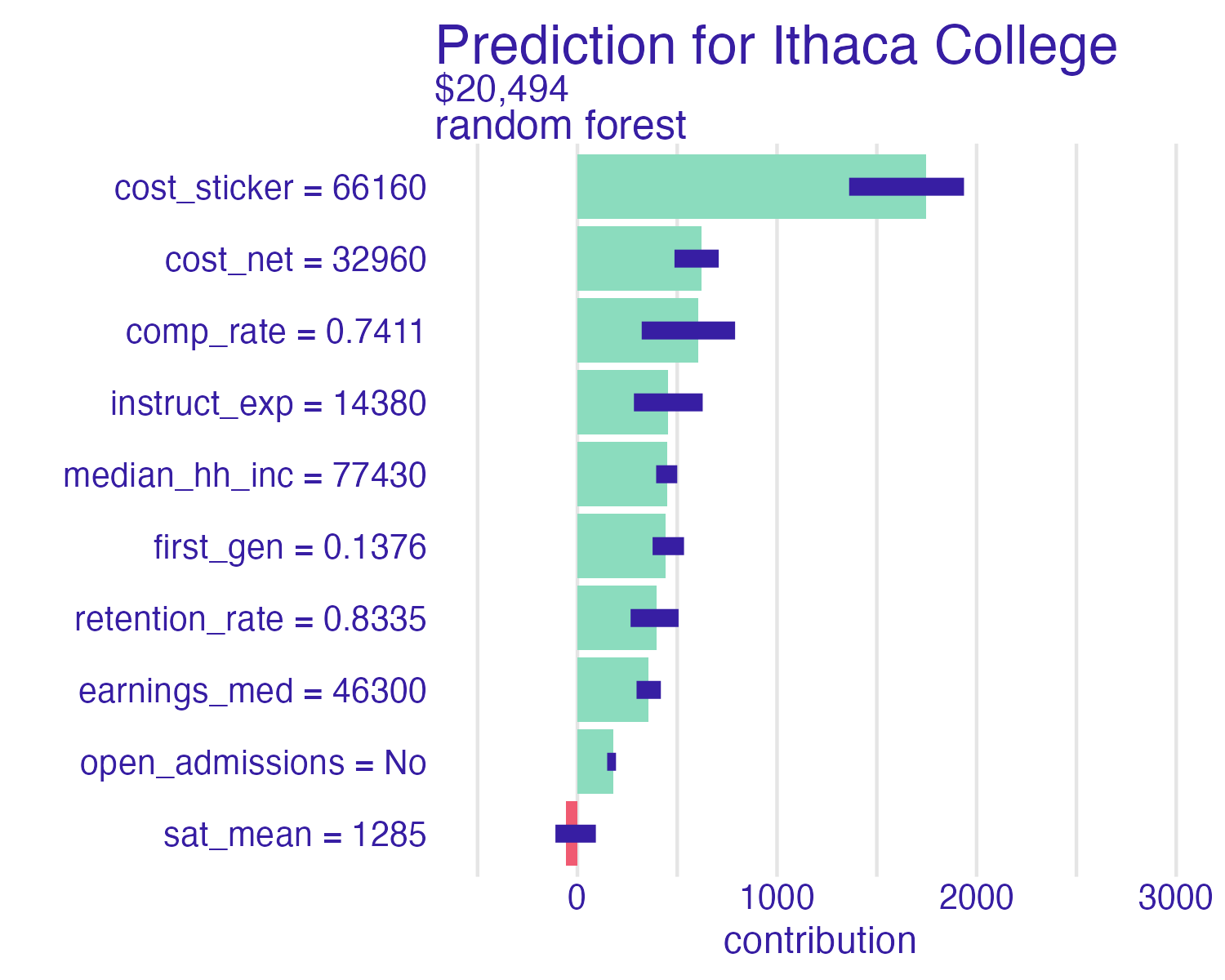
$ women_only <chr> "No"Ithaca College
Rows: 1
Columns: 26
$ state               <chr> "NY"
$ act_med             <dbl> NA
$ adm_rate            <dbl> 0.6994
$ comp_rate           <dbl> 0.7411
$ cost_net            <dbl> 32965
$ cost_sticker        <dbl> 66162
$ death_pct           <dbl> NA
$ debt                <dbl> 19500
$ earnings_med        <dbl> 46305
$ earnings_sd         <dbl> 33036
$ faculty_full_time   <dbl> 0.7583
$ faculty_salary_mean <dbl> 86337
$ female              <dbl> 0.5863059
$ first_gen           <dbl> 0.1375752
$ instruct_exp        <dbl> 14377
$ locale              <chr> "Suburb"
$ median_hh_inc       <dbl> 77434
$ open_admissions     <chr> "No"
$ pbi                 <chr> "No"
$ pell_pct            <dbl> 0.1901
$ retention_rate      <dbl> 0.8335
$ sat_mean            <dbl> 1285
$ test_policy         <chr> "Considered but not required"
$ type                <chr> "Private, nonprofit"
$ veteran             <dbl> NA
$ women_only          <chr> "No"
Breakdown methods
- How contributions attributed to individual features change the mean model’s prediction for a particular observation
- Sequentially fix the value of individual features and examine the change in the prediction
More info: Break-down Plots for Additive Attributions
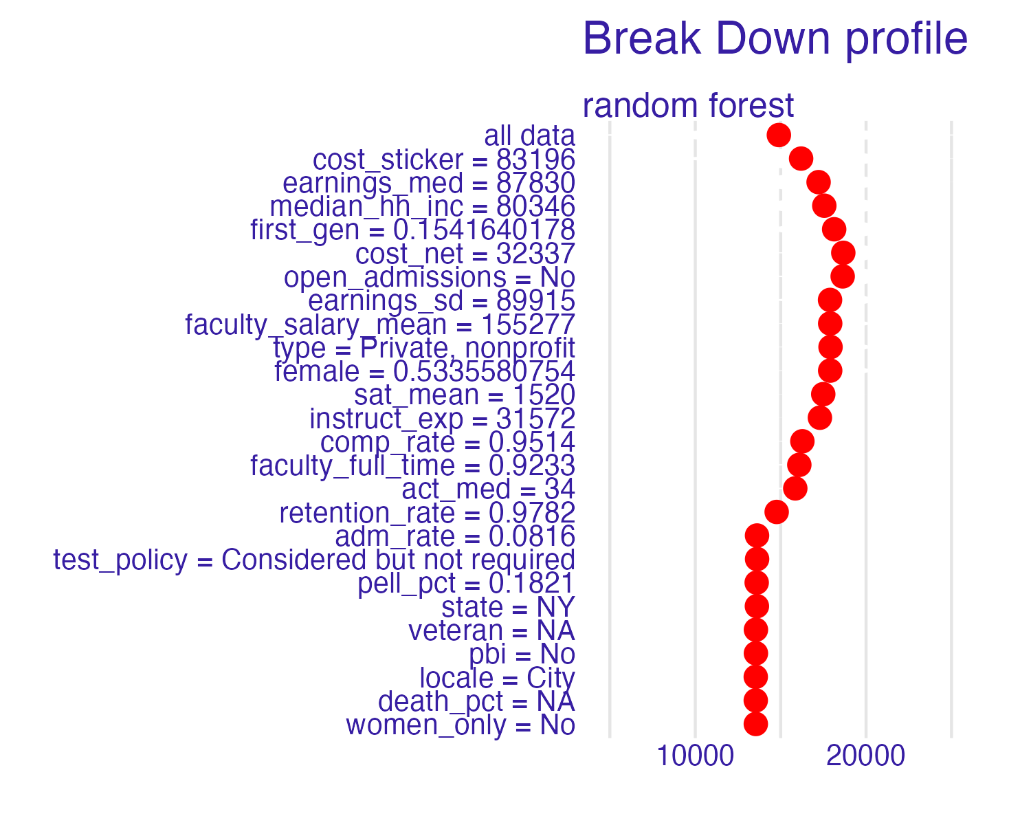
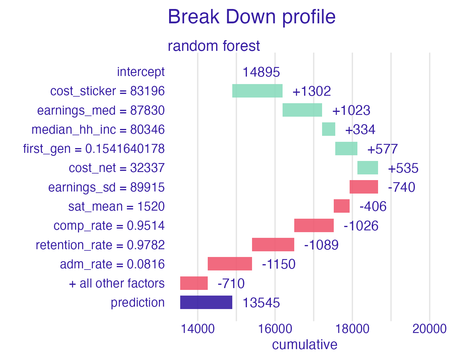
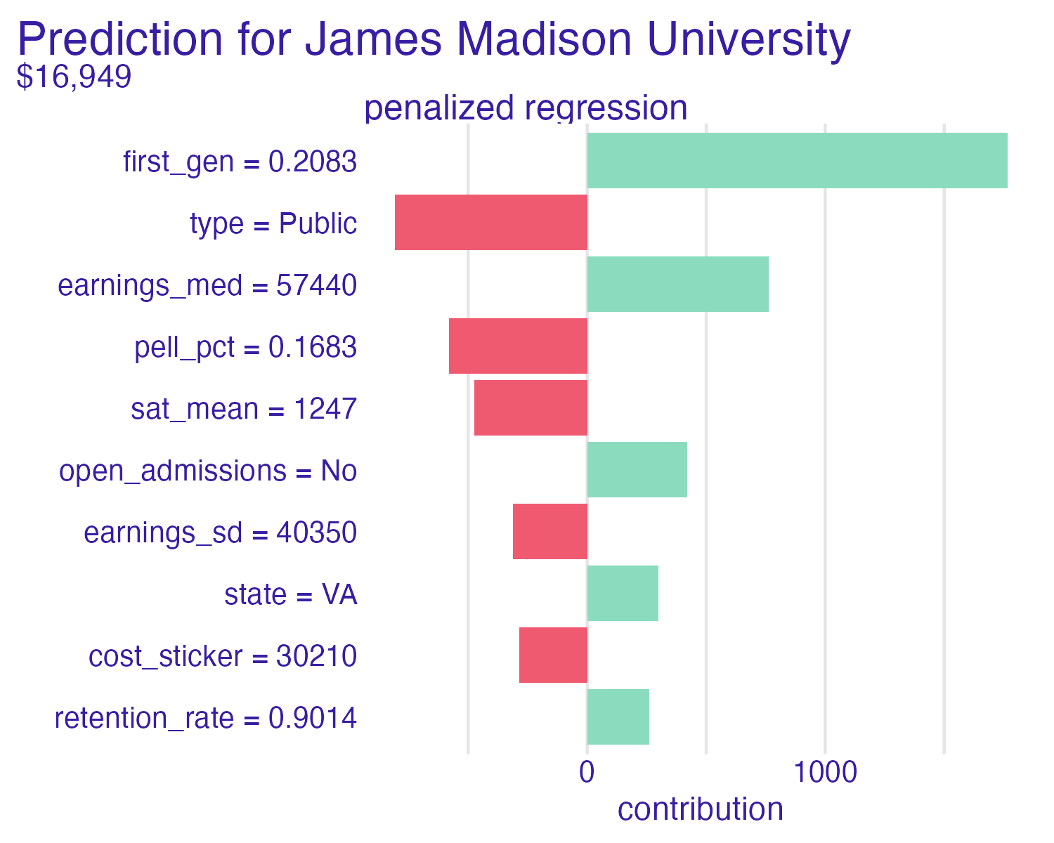
Breakdown of Cornell University using the random forest model
Code
📝 Break down the model
Which features contribute the most to the prediction for Cornell University? Which features contribute the least?
03:00
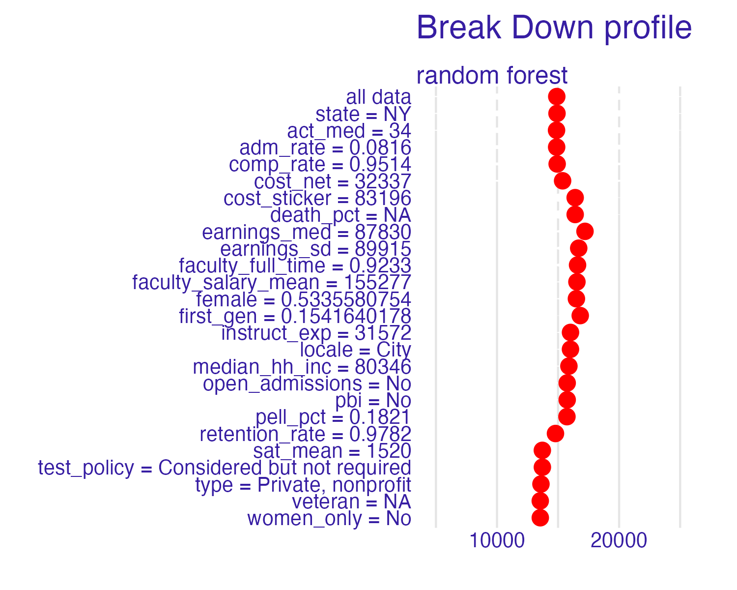
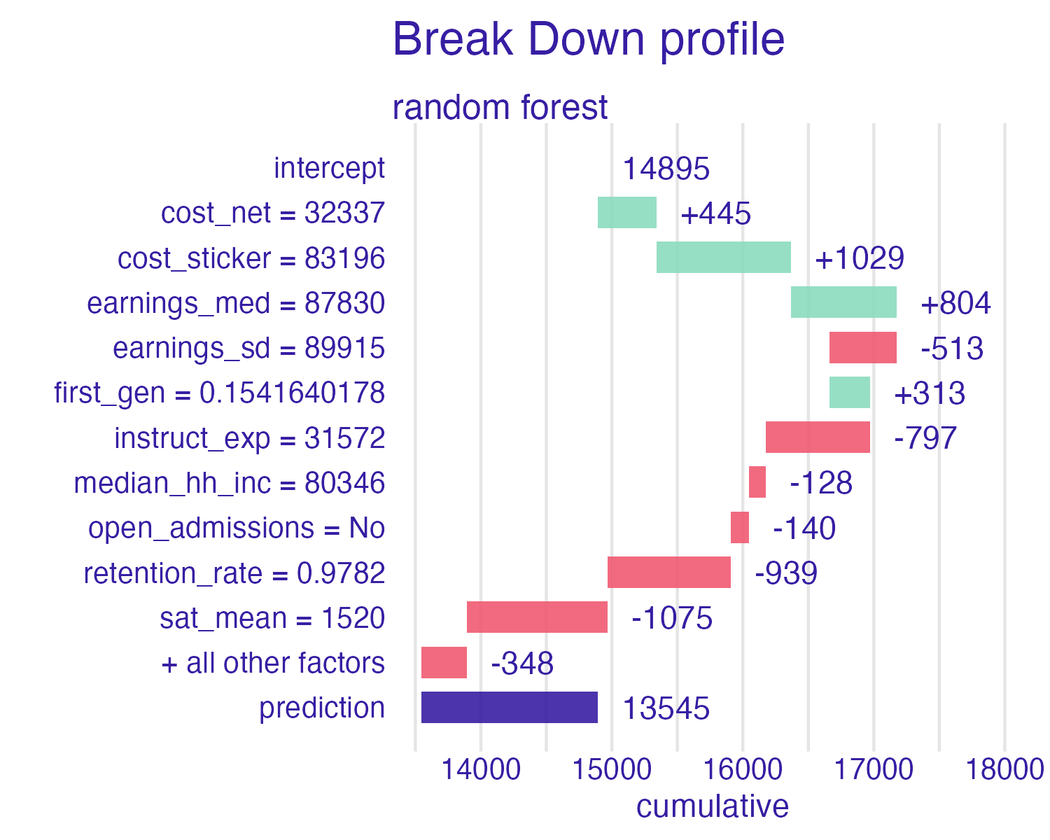
Breakdown of random forest
Breakdown plots
Advantages
- Easy to understand
- Compact visualization
- Intuitive explanation for linear models
Disadvantages
- Ignores interactive contributions (assumes everything is additive)
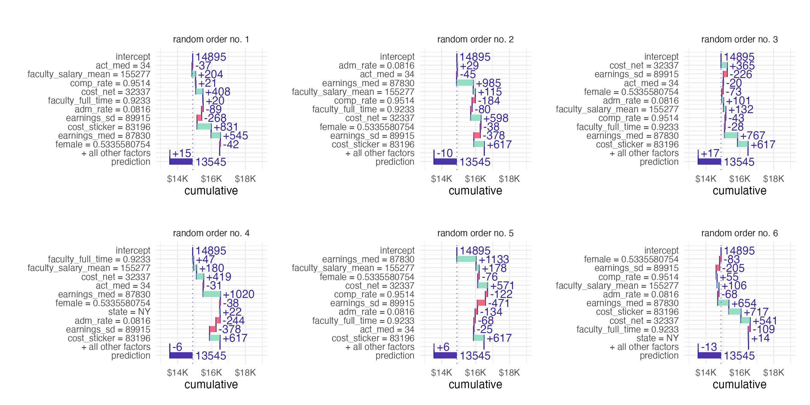
- Ordering of the explanatory variables influences the breakdown and resulting explanation
- Harder to interpret for models with lots of predictors
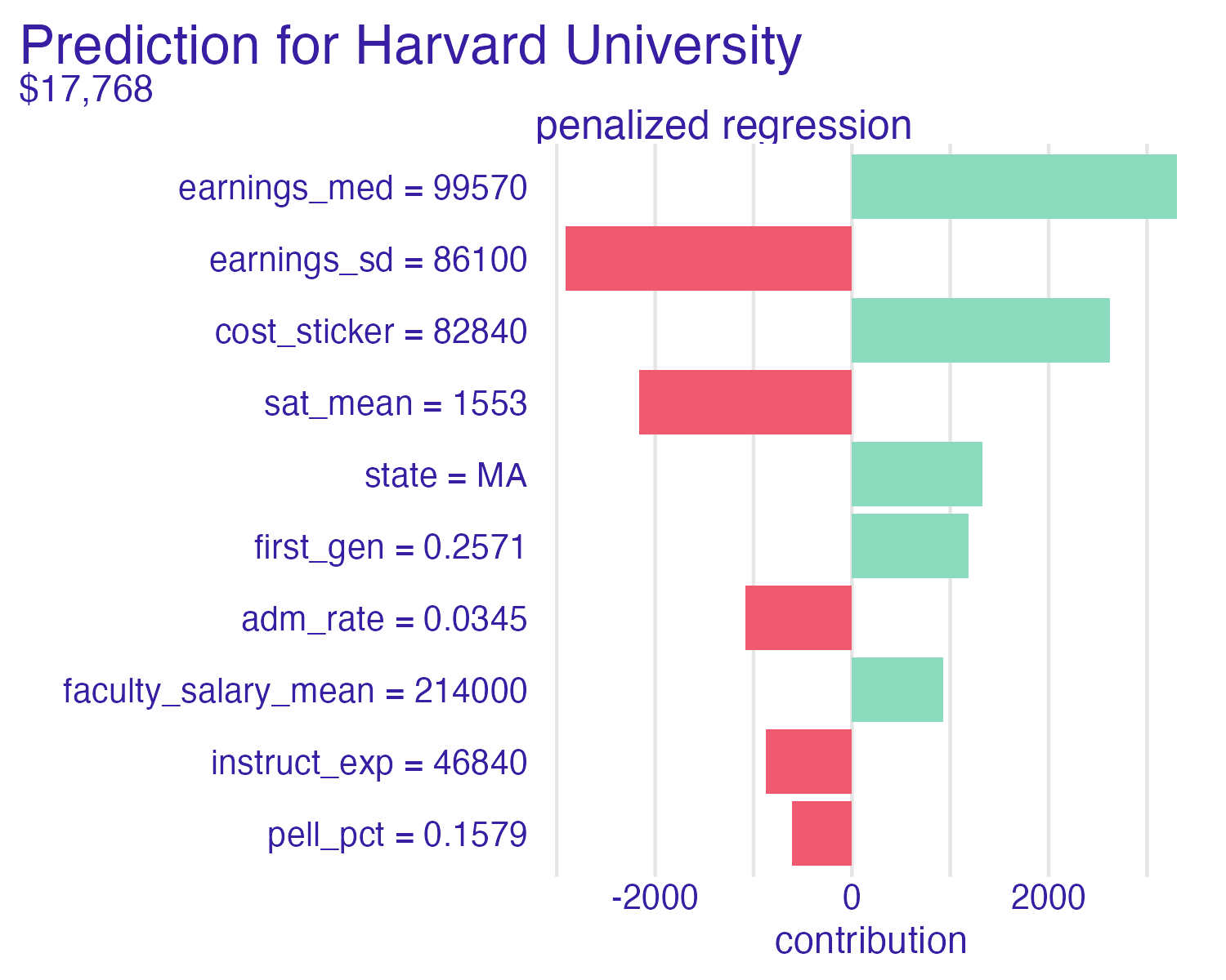
Shapley Additive Explanations (SHAP)
Shapley Additive Explanations (SHAP)
- Average contributions of features are computed under different coalitions of feature orderings
- Randomly permute feature order using \(B\) combinations
- Average across individual breakdowns to calculate feature contribution to individual prediction
SHAP for Cornell
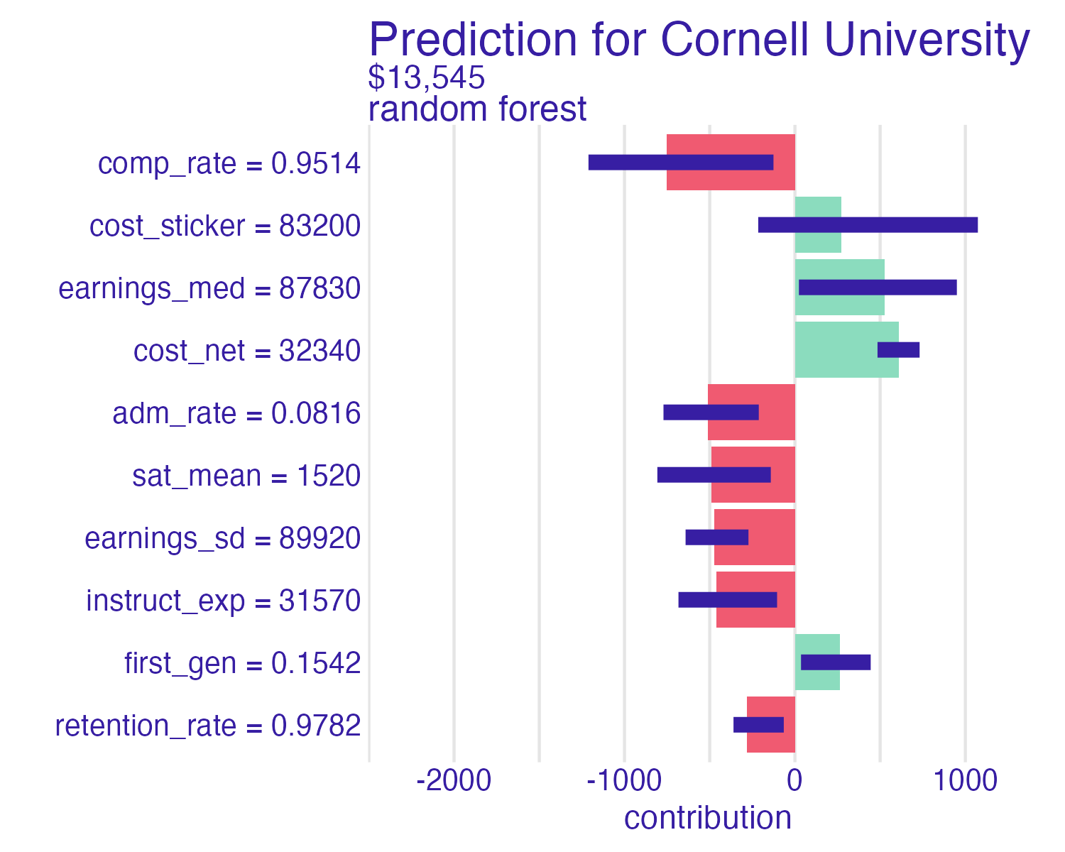
Cornell University vs. Ithaca College

Cornell University vs. Ithaca College

Shapley values
Advantages
- Model-agnostic
- Strong formal foundation from game theory
- Considers all (or many) possible feature orderings
Disadvantages
- Ignores interactive contributions (assumes everything is additive)
- Larger number of predictors makes it impossible to consider all possible coalitions
- Computationally expensive
📝 Interpreting Shapley values
Instructions
Interpret the Shapley values for the schools below. How do the predictions compare? Which features contribute the most to the predictions? How do the contributions differ between schools?
06:00
Global explanations
Understand which features are most important in driving the predictions of the models overall, aggregated across the training set
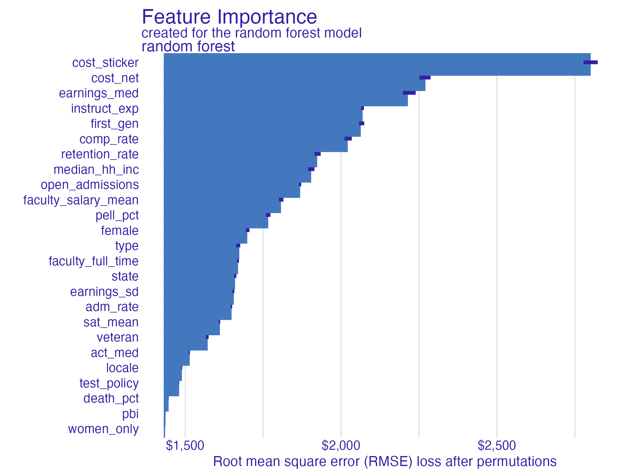
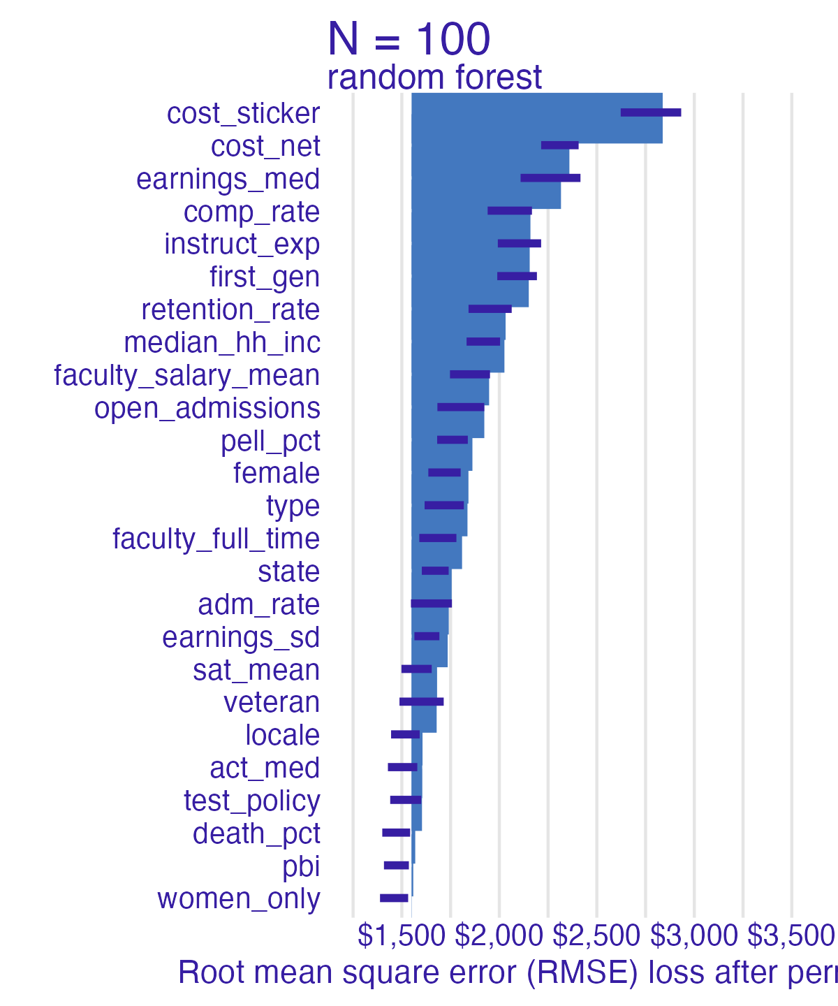
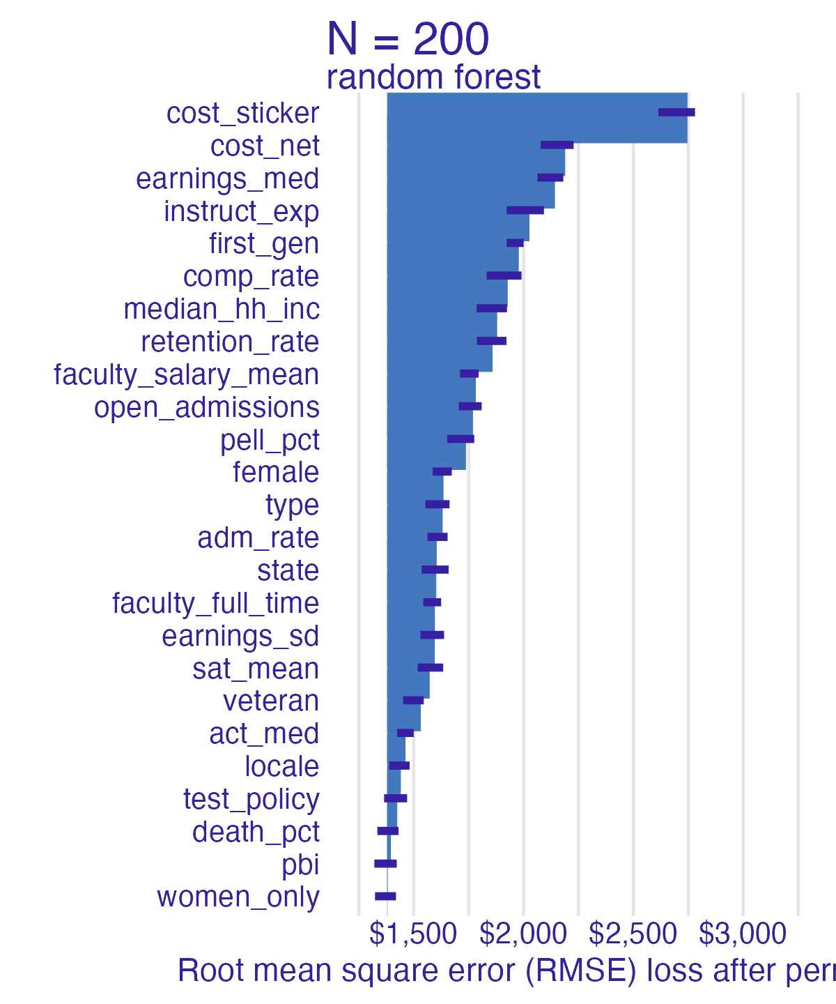
Feature importance
Feature importance
- Relative importance of each feature in a dataset for predicting the outcome
- How each feature contributes to the model’s predictions
- Model-specific techniques
- Lasso regression
- Random forests
- Model-agnostic approach
Permutation-based feature importance
- Calculate the increase in the model’s prediction error after permuting the feature
- Randomly shuffle the feature’s values across observations
- Important feature
- Unimportant feature
For any given loss function do
1: compute loss function for original model
2: for variable i in {1,...,p} do
     | randomize values
     | apply given ML model
     | estimate loss function
     | compute feature importance (permuted loss / original loss)
   end
3. Sort variables by descending feature importance
More info: Permutation Feature Importance
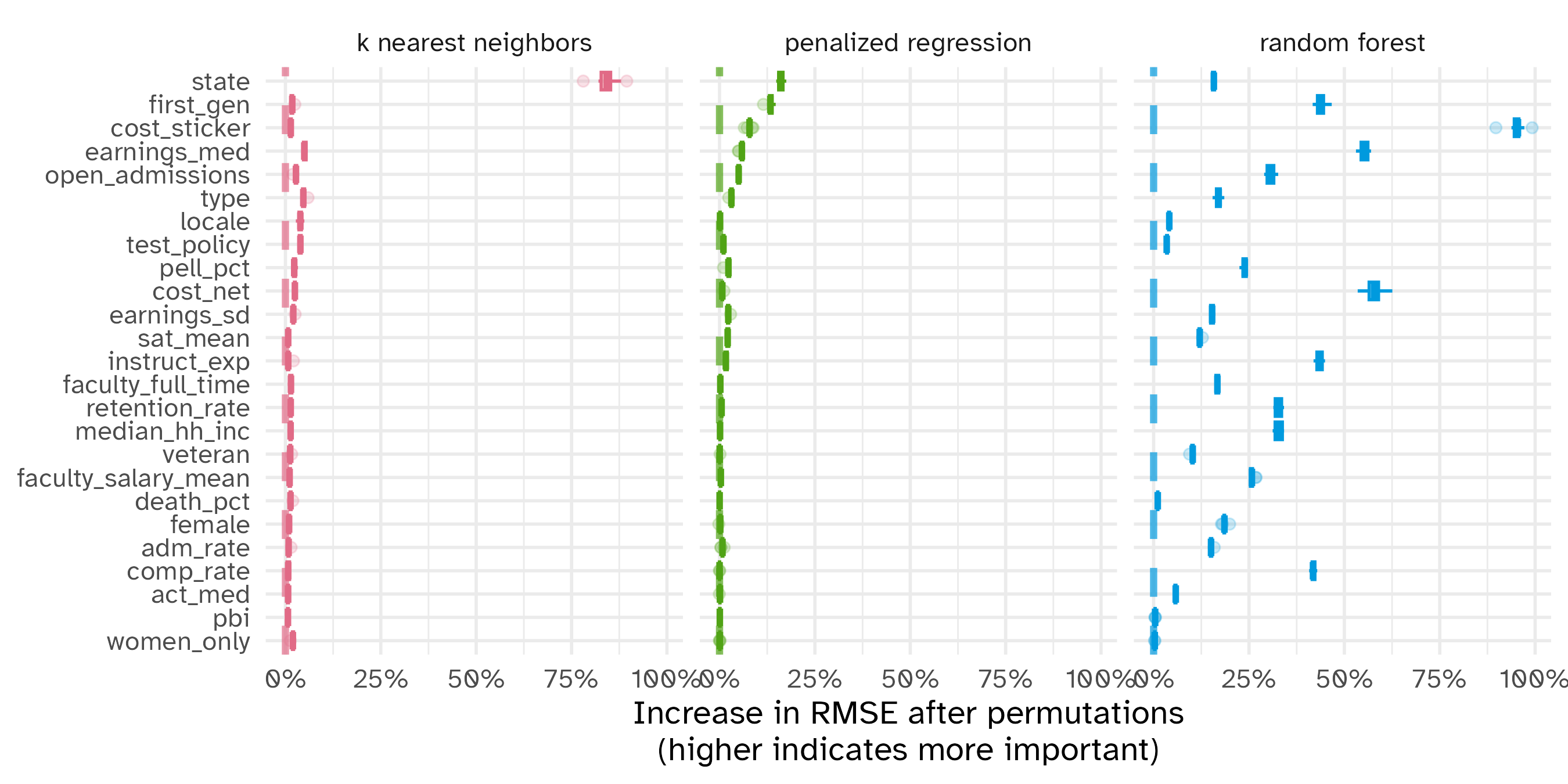
Random forest feature importance
Number of observations permuted
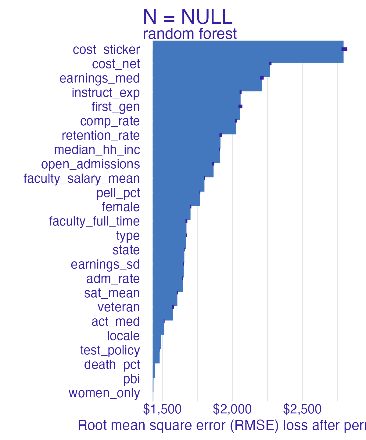
Measuring changes
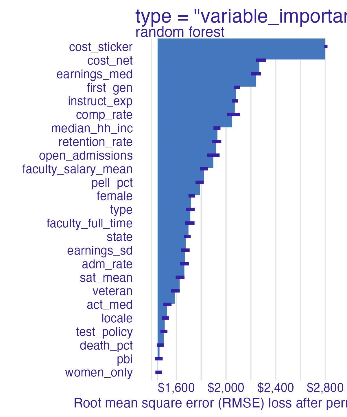

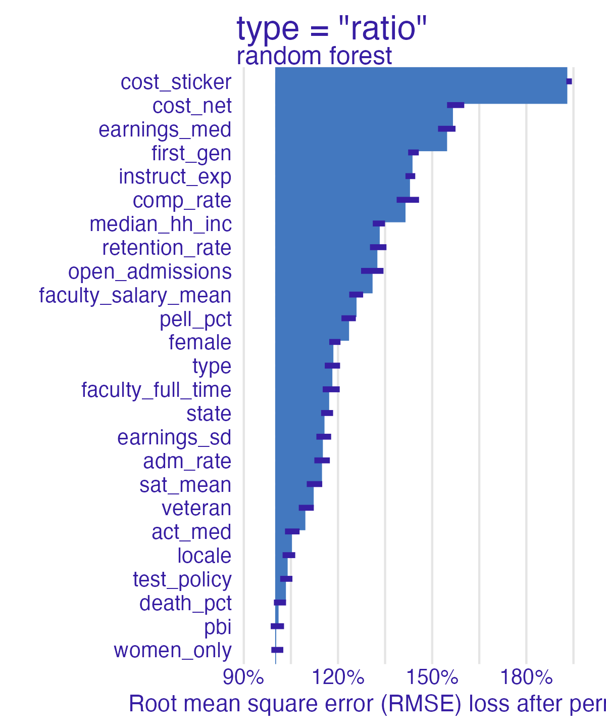
📝 Comparing feature importance
Instructions
- Which features are most/least important for predicting student debt?
- How does the model choice influence the relative importance of features?
06:00
Permutation-based feature importance
Advantages
- Clear interpretation
- Succinct measure
- Does not require retraining the model
- Takes into account all interactions
Disadvantages
- Permutation adds randomness to results - results may vary greatly
- Computationally expensive
- Linked to the error of the model
- Need access to the true outcome
- Takes into account all interactions
Building global explanations from local explanations
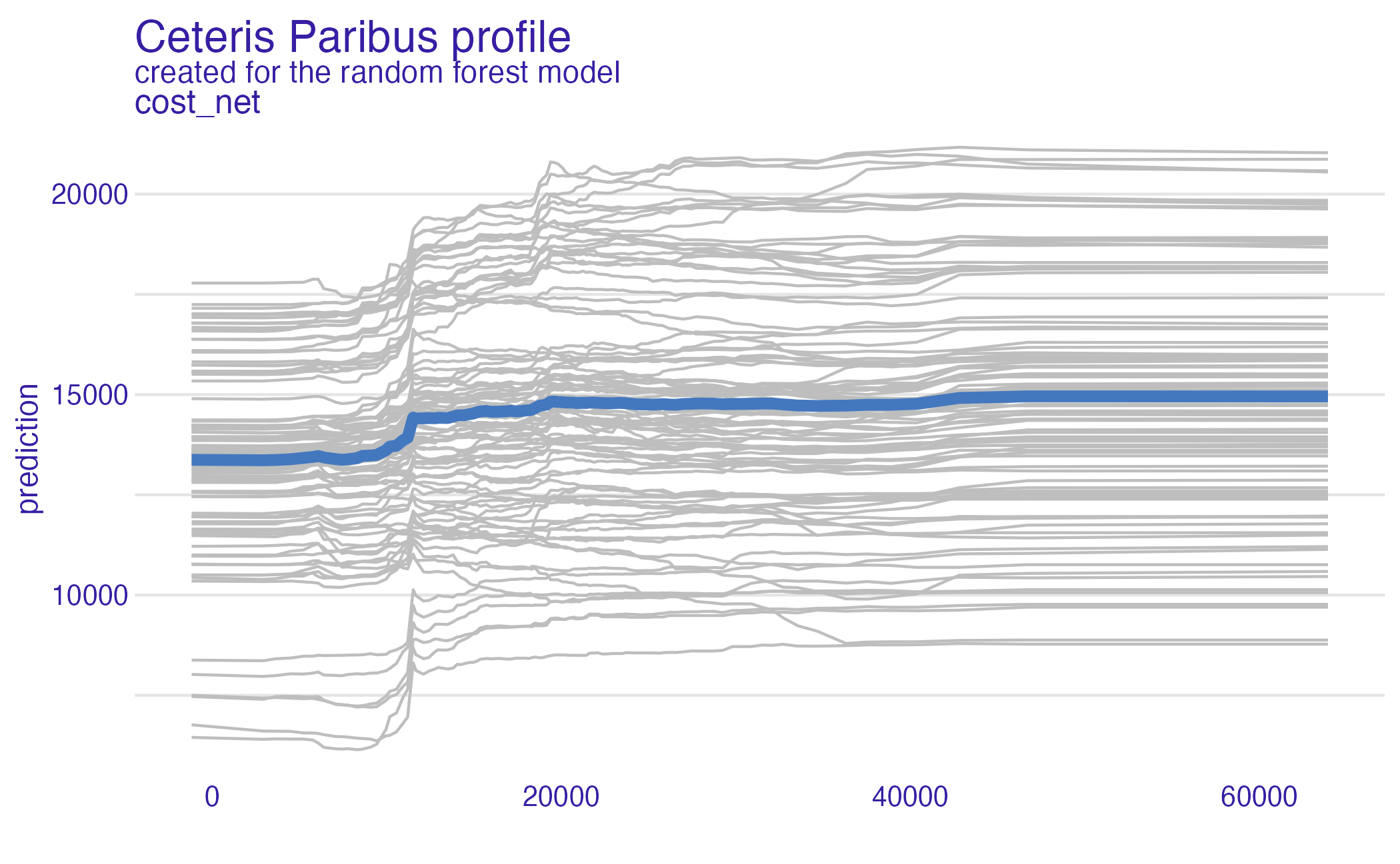
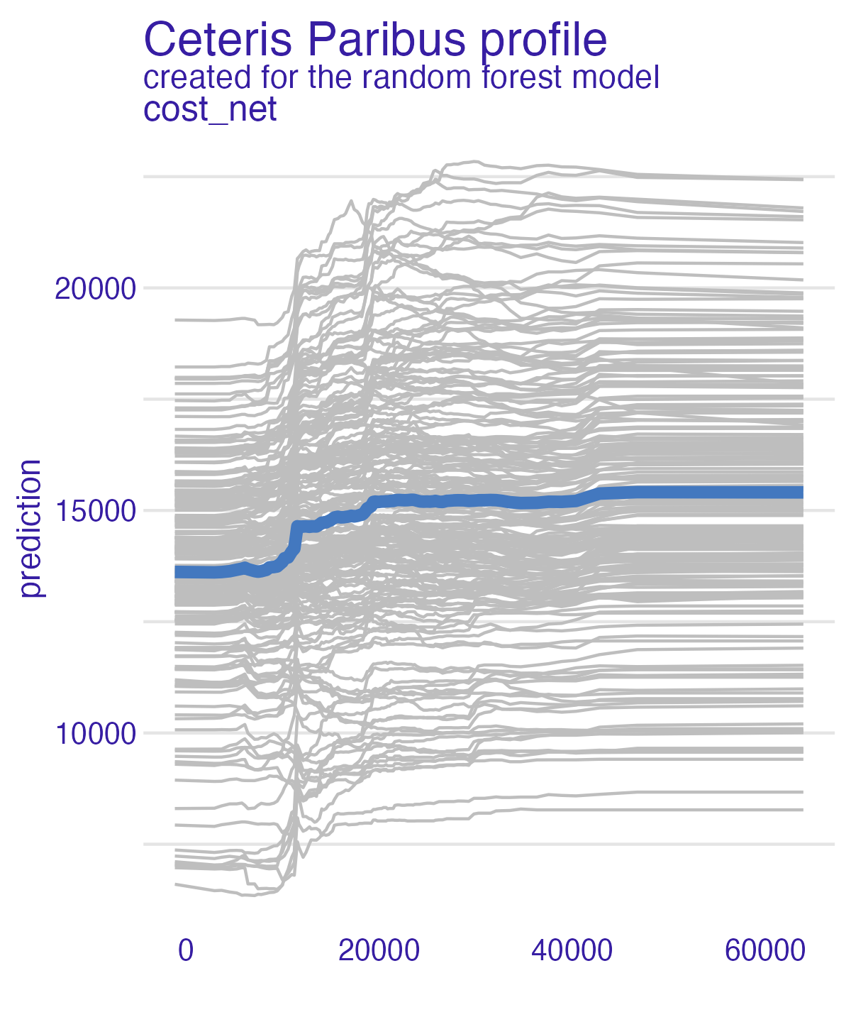
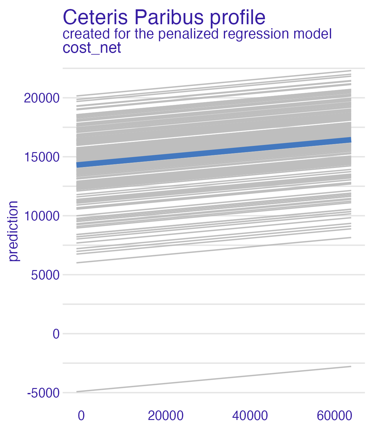
Individual conditional expectation (ICE 😬)
- Ceteris peribus - “other things held constant”
- Marginal effect a feature has on the predictor
- Counterfactual comparison - what if this observation had \(Y\) value instead of \(X\)?
- Plot one observation that shows how the observation’s prediction changes when a feature changes
More info: Interpretable Machine Learning
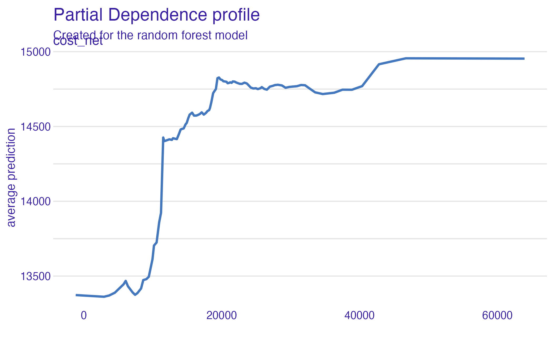
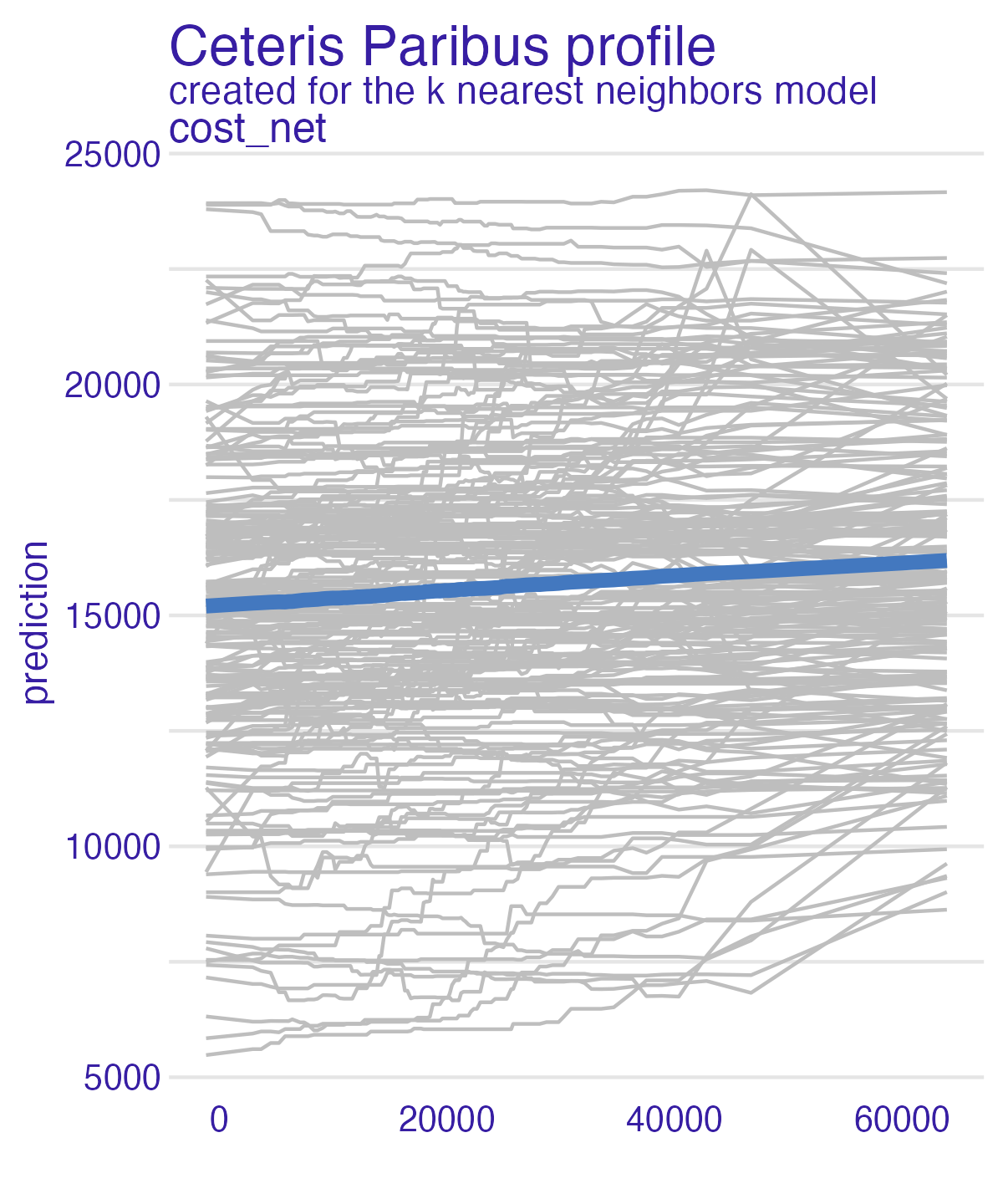
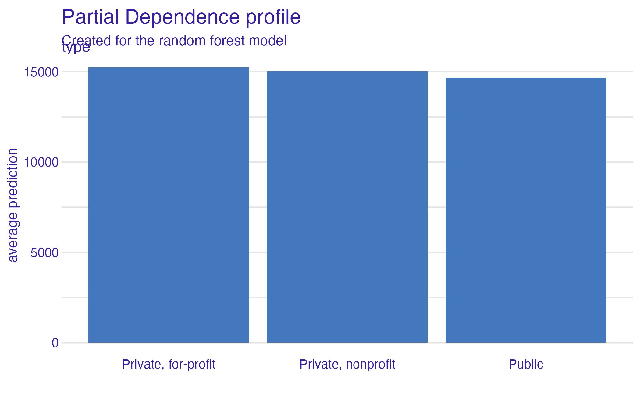
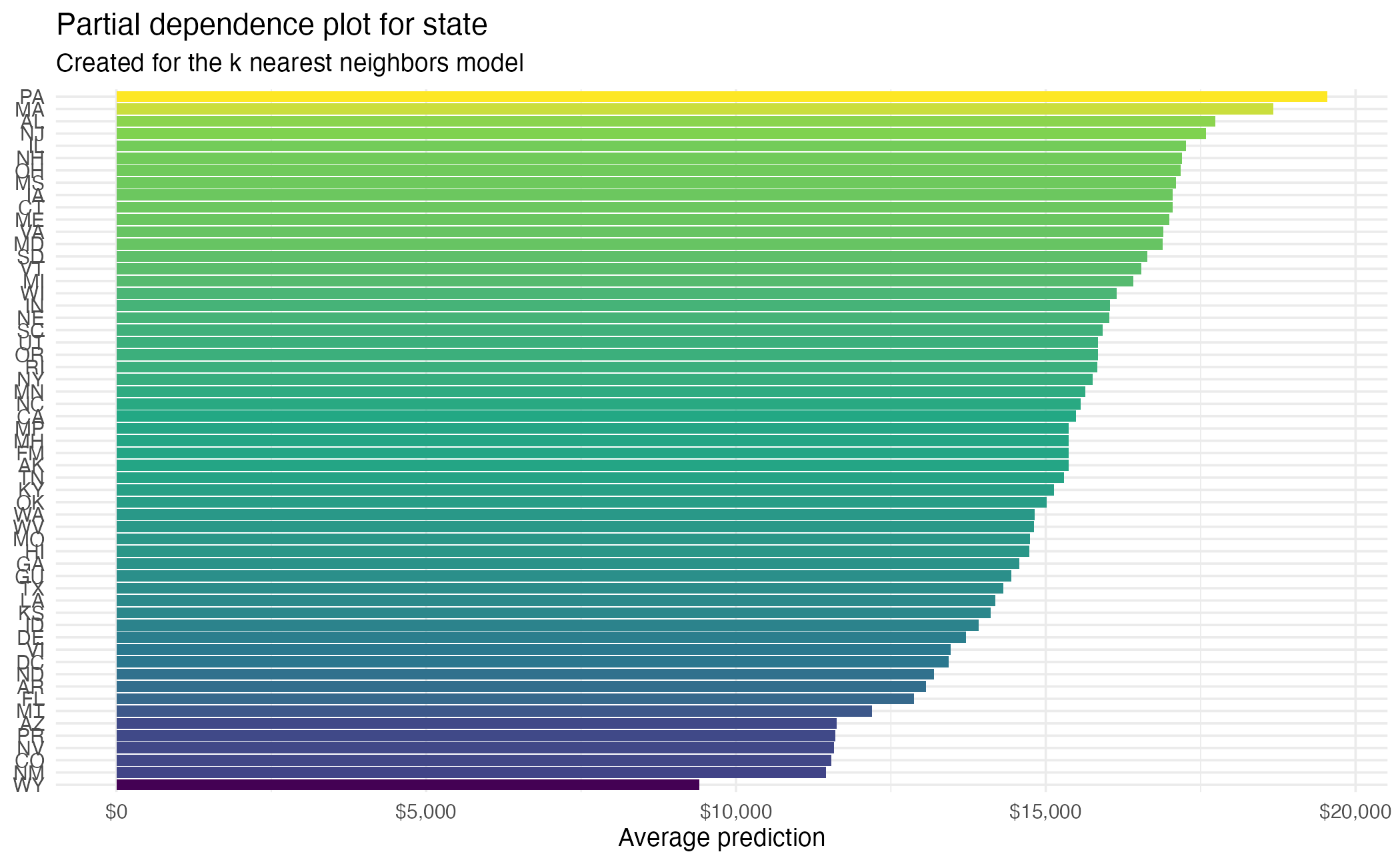
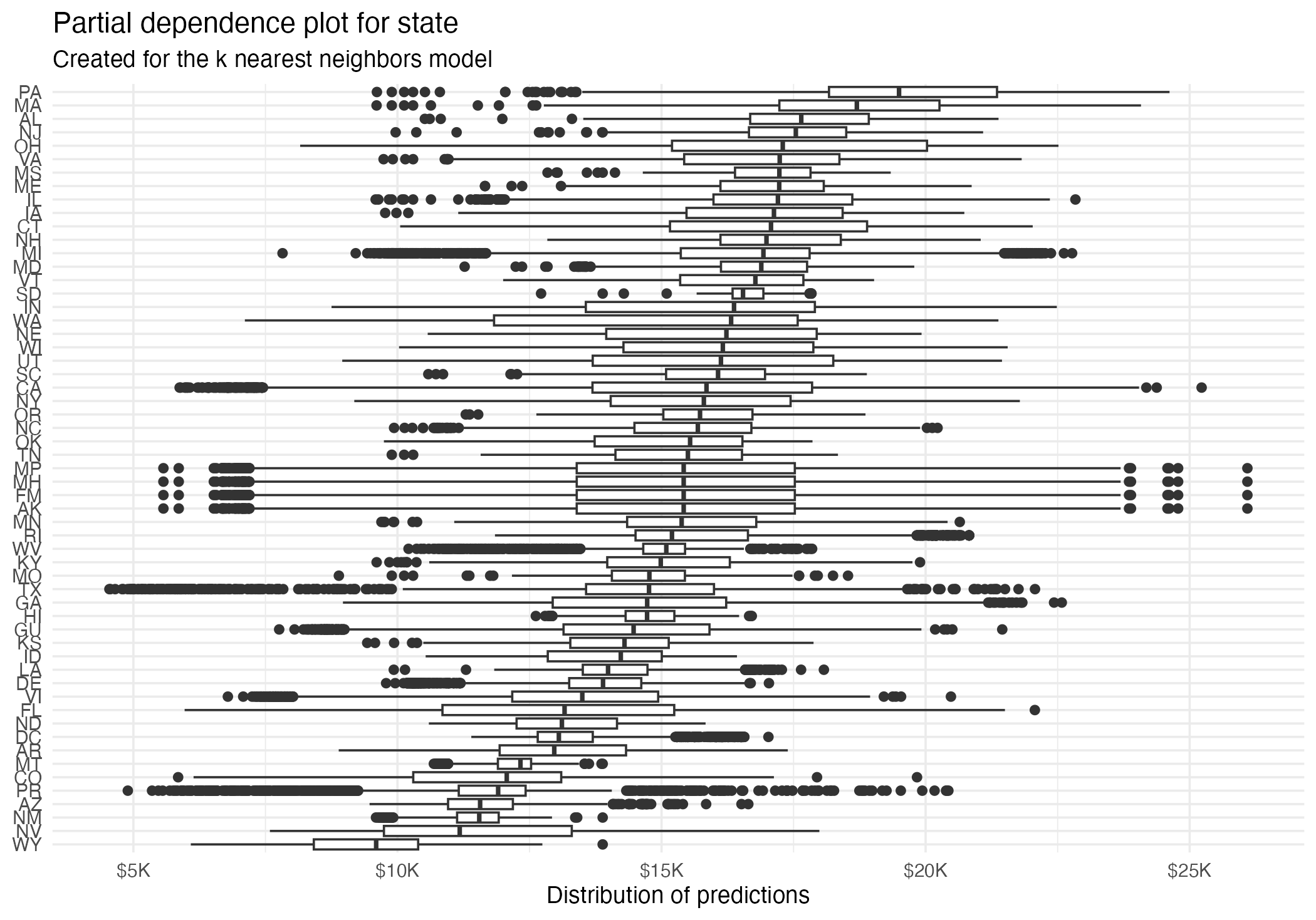
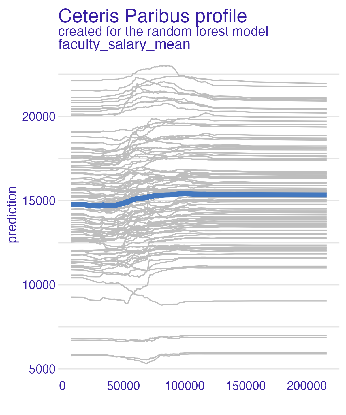
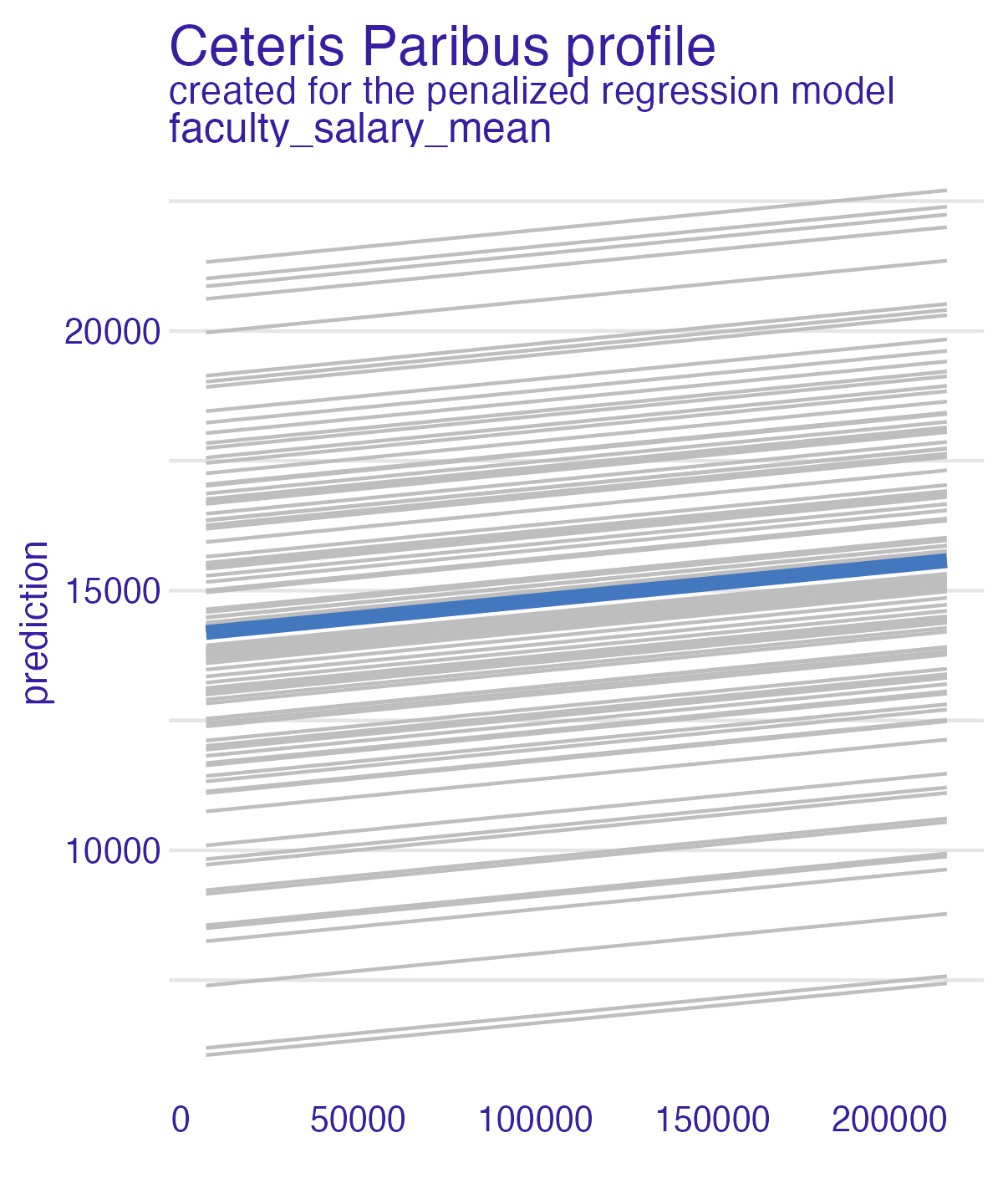
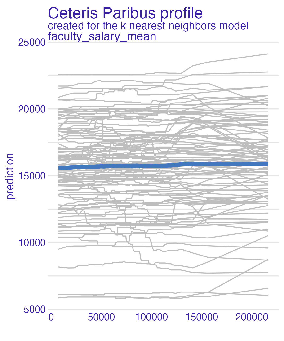
Partial dependence plot (PDP)
Average multiple ICEs to estimate the marginal effect of a feature on the outcome of interest
More info: Interpretable Machine Learning
Net cost (PDP)
Net cost (PDP + ICE)
Net cost (PDP + ICE) – all models
Type (PDP)
State (PDP)
State (PDP + ICE)
Partial dependence plot (PDP)
Advantages
- Intuitive
- Clear interpretation (assuming variables are uncorrelated)
- Straightforward implementation
Disadvantages
- Limited to one or two variables
- Assumes independence of features
- Heterogeneous effects might be hidden - add ICE curves to visualize heterogeneity
📝 Those pesky faculty
How does the average faculty salary influence the predictions of the debt models?
05:00
Wrap-up
Recap
- Explainability is crucial for understanding and trusting machine learning models
- Breakdown profiles and Shapley values provide local explanations for individual predictions
- Permutation-based feature importance provides insight into the importance of features in a model
- Partial dependence plots provide a global view of the relationship between a feature and the model’s predictions