AE 08: Explore coffee taste tests
The Great American Coffee Taste Test
In October 2023, James Hoffmann and coffee company Cometeer held the “Great American Coffee Taste Test” on YouTube, during which viewers were asked to fill out a survey about 4 coffees they ordered from Cometeer for the tasting. Tidy Tuesday published the data set we are using.
coffee_survey <- read_csv(file = "data/coffee_survey.csv")It includes the following features:
| variable | class | description |
|---|---|---|
| submission_id | character | Submission ID |
| age | character | What is your age? |
| cups | character | How many cups of coffee do you typically drink per day? |
| where_drink | character | Where do you typically drink coffee? |
| brew | character | How do you brew coffee at home? |
| brew_other | character | How else do you brew coffee at home? |
| purchase | character | On the go, where do you typically purchase coffee? |
| purchase_other | character | Where else do you purchase coffee? |
| favorite | character | What is your favorite coffee drink? |
| favorite_specify | character | Please specify what your favorite coffee drink is |
| additions | character | Do you usually add anything to your coffee? |
| additions_other | character | What else do you add to your coffee? |
| dairy | character | What kind of dairy do you add? |
| sweetener | character | What kind of sugar or sweetener do you add? |
| style | character | Before today’s tasting, which of the following best described what kind of coffee you like? |
| strength | character | How strong do you like your coffee? |
| roast_level | character | What roast level of coffee do you prefer? |
| caffeine | character | How much caffeine do you like in your coffee? |
| expertise | numeric | Lastly, how would you rate your own coffee expertise? |
| coffee_a_bitterness | numeric | Coffee A - Bitterness |
| coffee_a_acidity | numeric | Coffee A - Acidity |
| coffee_a_personal_preference | numeric | Coffee A - Personal Preference |
| coffee_a_notes | character | Coffee A - Notes |
| coffee_b_bitterness | numeric | Coffee B - Bitterness |
| coffee_b_acidity | numeric | Coffee B - Acidity |
| coffee_b_personal_preference | numeric | Coffee B - Personal Preference |
| coffee_b_notes | character | Coffee B - Notes |
| coffee_c_bitterness | numeric | Coffee C - Bitterness |
| coffee_c_acidity | numeric | Coffee C - Acidity |
| coffee_c_personal_preference | numeric | Coffee C - Personal Preference |
| coffee_c_notes | character | Coffee C - Notes |
| coffee_d_bitterness | numeric | Coffee D - Bitterness |
| coffee_d_acidity | numeric | Coffee D - Acidity |
| coffee_d_personal_preference | numeric | Coffee D - Personal Preference |
| coffee_d_notes | character | Coffee D - Notes |
| prefer_abc | character | Between Coffee A, Coffee B, and Coffee C which did you prefer? |
| prefer_ad | character | Between Coffee A and Coffee D, which did you prefer? |
| prefer_overall | character | Lastly, what was your favorite overall coffee? |
| wfh | character | Do you work from home or in person? |
| total_spend | character | In total, much money do you typically spend on coffee in a month? |
| why_drink | character | Why do you drink coffee? |
| why_drink_other | character | Other reason for drinking coffee |
| taste | character | Do you like the taste of coffee? |
| know_source | character | Do you know where your coffee comes from? |
| most_paid | character | What is the most you’ve ever paid for a cup of coffee? |
| most_willing | character | What is the most you’d ever be willing to pay for a cup of coffee? |
| value_cafe | character | Do you feel like you’re getting good value for your money when you buy coffee at a cafe? |
| spent_equipment | character | Approximately how much have you spent on coffee equipment in the past 5 years? |
| value_equipment | character | Do you feel like you’re getting good value for your money when you buy coffee at a cafe? |
| gender | character | Gender |
| gender_specify | character | Gender (please specify) |
| education_level | character | Education Level |
| ethnicity_race | character | Ethnicity/Race |
| ethnicity_race_specify | character | Ethnicity/Race (please specify) |
| employment_status | character | Employment Status |
| number_children | character | Number of Children |
| political_affiliation | character | Political Affiliation |
Our ultimate goal on the next homework assignment is to predict which coffee a respondent will prefer based on their survey responses. We will use the prefer_overall variable as our target.
A quick {skimr} of the data:
skim(coffee_survey)| Name | coffee_survey |
| Number of rows | 4042 |
| Number of columns | 57 |
| _______________________ | |
| Column type frequency: | |
| character | 44 |
| numeric | 13 |
| ________________________ | |
| Group variables | None |
Variable type: character
| skim_variable | n_missing | complete_rate | min | max | empty | n_unique | whitespace |
|---|---|---|---|---|---|---|---|
| submission_id | 0 | 1.00 | 6 | 6 | 0 | 4042 | 0 |
| age | 31 | 0.99 | 13 | 15 | 0 | 7 | 0 |
| cups | 93 | 0.98 | 1 | 11 | 0 | 6 | 0 |
| where_drink | 70 | 0.98 | 7 | 44 | 0 | 65 | 0 |
| brew | 385 | 0.90 | 5 | 165 | 0 | 449 | 0 |
| brew_other | 3364 | 0.17 | 2 | 319 | 0 | 160 | 0 |
| purchase | 3332 | 0.18 | 5 | 107 | 0 | 89 | 0 |
| purchase_other | 4011 | 0.01 | 4 | 83 | 0 | 26 | 0 |
| favorite | 62 | 0.98 | 5 | 32 | 0 | 12 | 0 |
| favorite_specify | 3926 | 0.03 | 3 | 92 | 0 | 78 | 0 |
| additions | 83 | 0.98 | 5 | 100 | 0 | 53 | 0 |
| additions_other | 3994 | 0.01 | 3 | 140 | 0 | 42 | 0 |
| dairy | 2356 | 0.42 | 8 | 110 | 0 | 175 | 0 |
| sweetener | 3530 | 0.13 | 5 | 99 | 0 | 82 | 0 |
| style | 84 | 0.98 | 4 | 11 | 0 | 12 | 0 |
| strength | 126 | 0.97 | 4 | 15 | 0 | 5 | 0 |
| roast_level | 102 | 0.97 | 4 | 7 | 0 | 7 | 0 |
| caffeine | 125 | 0.97 | 5 | 13 | 0 | 3 | 0 |
| coffee_a_notes | 1464 | 0.64 | 1 | 377 | 0 | 2317 | 0 |
| coffee_b_notes | 1586 | 0.61 | 1 | 980 | 0 | 2199 | 0 |
| coffee_c_notes | 1659 | 0.59 | 1 | 438 | 0 | 2163 | 0 |
| coffee_d_notes | 1454 | 0.64 | 1 | 528 | 0 | 2354 | 0 |
| prefer_abc | 270 | 0.93 | 8 | 8 | 0 | 3 | 0 |
| prefer_ad | 281 | 0.93 | 8 | 8 | 0 | 2 | 0 |
| prefer_overall | 272 | 0.93 | 8 | 8 | 0 | 4 | 0 |
| wfh | 518 | 0.87 | 18 | 26 | 0 | 3 | 0 |
| total_spend | 531 | 0.87 | 4 | 8 | 0 | 6 | 0 |
| why_drink | 474 | 0.88 | 5 | 93 | 0 | 84 | 0 |
| why_drink_other | 3875 | 0.04 | 2 | 195 | 0 | 163 | 0 |
| taste | 479 | 0.88 | 2 | 3 | 0 | 2 | 0 |
| know_source | 483 | 0.88 | 2 | 3 | 0 | 2 | 0 |
| most_paid | 515 | 0.87 | 5 | 13 | 0 | 8 | 0 |
| most_willing | 532 | 0.87 | 5 | 13 | 0 | 8 | 0 |
| value_cafe | 542 | 0.87 | 2 | 3 | 0 | 2 | 0 |
| spent_equipment | 536 | 0.87 | 7 | 16 | 0 | 7 | 0 |
| value_equipment | 548 | 0.86 | 2 | 3 | 0 | 2 | 0 |
| gender | 519 | 0.87 | 4 | 22 | 0 | 5 | 0 |
| gender_specify | 4030 | 0.00 | 2 | 28 | 0 | 11 | 0 |
| education_level | 604 | 0.85 | 15 | 34 | 0 | 6 | 0 |
| ethnicity_race | 624 | 0.85 | 15 | 29 | 0 | 6 | 0 |
| ethnicity_race_specify | 3937 | 0.03 | 2 | 53 | 0 | 82 | 0 |
| employment_status | 623 | 0.85 | 7 | 18 | 0 | 6 | 0 |
| number_children | 636 | 0.84 | 1 | 11 | 0 | 5 | 0 |
| political_affiliation | 753 | 0.81 | 8 | 14 | 0 | 4 | 0 |
Variable type: numeric
| skim_variable | n_missing | complete_rate | mean | sd | p0 | p25 | p50 | p75 | p100 | hist |
|---|---|---|---|---|---|---|---|---|---|---|
| expertise | 104 | 0.97 | 5.69 | 1.95 | 1 | 5 | 6 | 7 | 10 | ▂▃▇▇▁ |
| coffee_a_bitterness | 244 | 0.94 | 2.14 | 0.95 | 1 | 1 | 2 | 3 | 5 | ▅▇▃▂▁ |
| coffee_a_acidity | 263 | 0.93 | 3.63 | 0.98 | 1 | 3 | 4 | 4 | 5 | ▁▂▅▇▃ |
| coffee_a_personal_preference | 253 | 0.94 | 3.31 | 1.19 | 1 | 2 | 3 | 4 | 5 | ▂▅▆▇▅ |
| coffee_b_bitterness | 262 | 0.94 | 3.01 | 0.99 | 1 | 2 | 3 | 4 | 5 | ▂▅▇▆▁ |
| coffee_b_acidity | 275 | 0.93 | 2.22 | 0.87 | 1 | 2 | 2 | 3 | 5 | ▃▇▅▁▁ |
| coffee_b_personal_preference | 269 | 0.93 | 3.07 | 1.11 | 1 | 2 | 3 | 4 | 5 | ▂▆▇▆▃ |
| coffee_c_bitterness | 278 | 0.93 | 3.07 | 1.00 | 1 | 2 | 3 | 4 | 5 | ▁▅▇▆▂ |
| coffee_c_acidity | 291 | 0.93 | 2.37 | 0.92 | 1 | 2 | 2 | 3 | 5 | ▃▇▆▂▁ |
| coffee_c_personal_preference | 276 | 0.93 | 3.06 | 1.13 | 1 | 2 | 3 | 4 | 5 | ▂▆▇▆▃ |
| coffee_d_bitterness | 275 | 0.93 | 2.16 | 1.08 | 1 | 1 | 2 | 3 | 5 | ▇▇▅▂▁ |
| coffee_d_acidity | 277 | 0.93 | 3.86 | 1.01 | 1 | 3 | 4 | 5 | 5 | ▁▂▃▇▆ |
| coffee_d_personal_preference | 278 | 0.93 | 3.38 | 1.45 | 1 | 2 | 4 | 5 | 5 | ▅▃▃▆▇ |
Examining continuous variables
Your turn: Examine expertise using a histogram and appropriate binwidth. Describe the features of this variable.
# add code hereAdd response here.
Your turn: Each coffee has three numeric ratings by the respondents: bitterness, acidity, and personal preference. Create a histogram for each of these characteristics, faceted by coffee type. What do you notice?
The original structure of the data is one column for each coffee for each characteristic. You could create separate graphs for each of the 12 columns, but that seems like a lot of work. Instead, consider using the pivot_longer() function to restructure the data to one row per coffee per characteristic. This will make it easier to create the faceted histograms.
coffee_survey |>
  select(starts_with("coffee"), -ends_with("notes")) |>
  pivot_longer(
    cols = everything(),
    names_to = c("coffee", "measure"),
    names_prefix = "coffee_",
    names_sep = "_",
    values_to = "value"
  )
# A tibble: 48,504 × 3
coffee measure value
<chr> <chr> <dbl>
1 a bitterness NA
2 a acidity NA
3 a personal NA
4 b bitterness NA
5 b acidity NA
6 b personal NA
7 c bitterness NA
8 c acidity NA
9 c personal NA
10 d bitterness NA
# ℹ 48,494 more rows# add code hereAdd response here.
Examining categorical variables
Your turn: Examine prefer_overall graphically. Record your observations.
# add code hereAdd response here.
Your turn: Examine cups, brew, and roast_level. Record your observations, in particular how you might need to handle these variables in the modeling stage.
# add code hereAdd response here.
# add code hereAdd response here.
# add code hereAdd response here.
Making comparisons
Your turn: Compare the relationship between overall preference and the respondents’ preferred roast levels. Use a proportional bar chart to visualize the relationship.
Use position = "fill" with geom_bar() to automatically calculate percentages for the chart.
# add code hereAdd response here.
Your turn: Examine the relationship between the respondents’ numeric ratings for acidity, bitterness, and personal preference for each of the four coffees and compare to their overall preference. Record your observations.
Add response here.
Data quality
Missingness
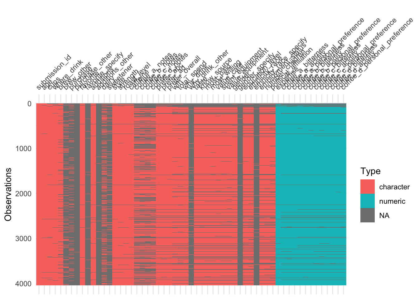
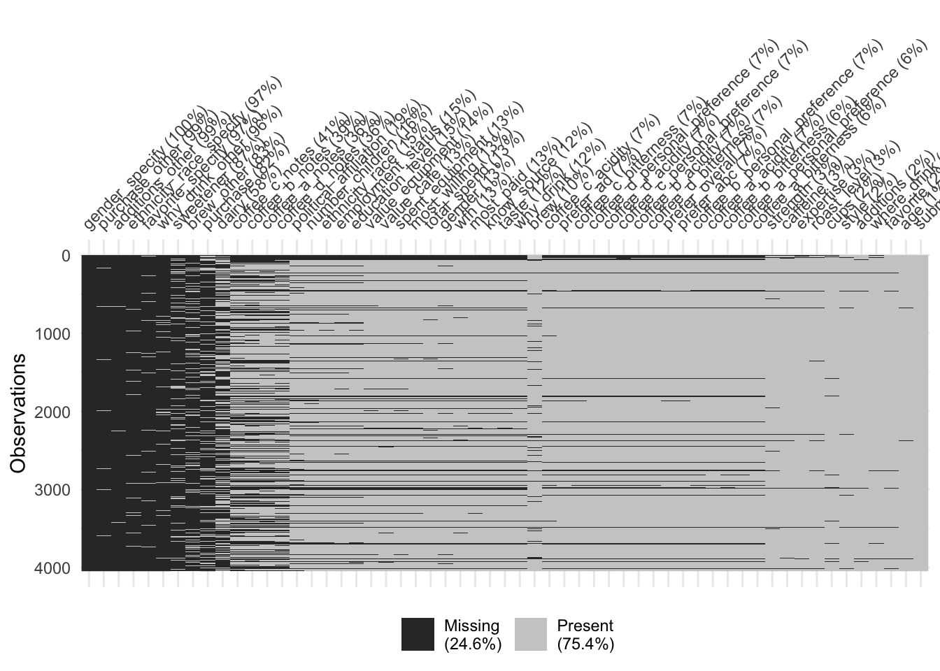
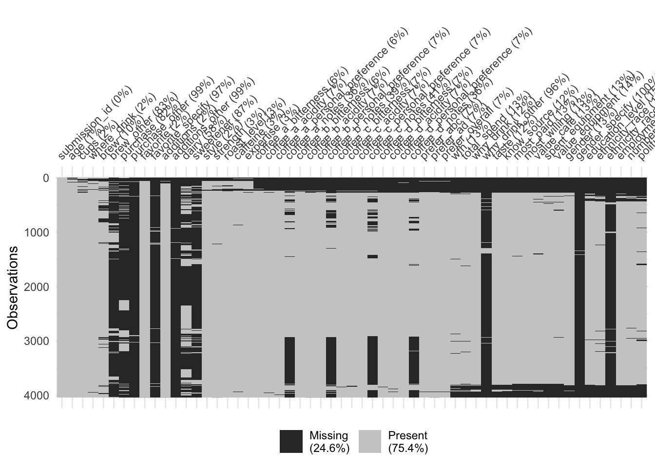
Demonstration: Use {visdat} to visualize missingness patterns in the data set.
# reorder columns based on % missing
vis_miss(coffee_survey, sort_miss = TRUE)
# cluster rows based on similarity in missingness patterns
vis_miss(coffee_survey, cluster = TRUE)Your turn: Record your observations on the missingness patterns in the data set. What variables have high missingness? Is this surprising? What might you do to variables or observations with high degrees of missingness?
Add response here.
Outliers
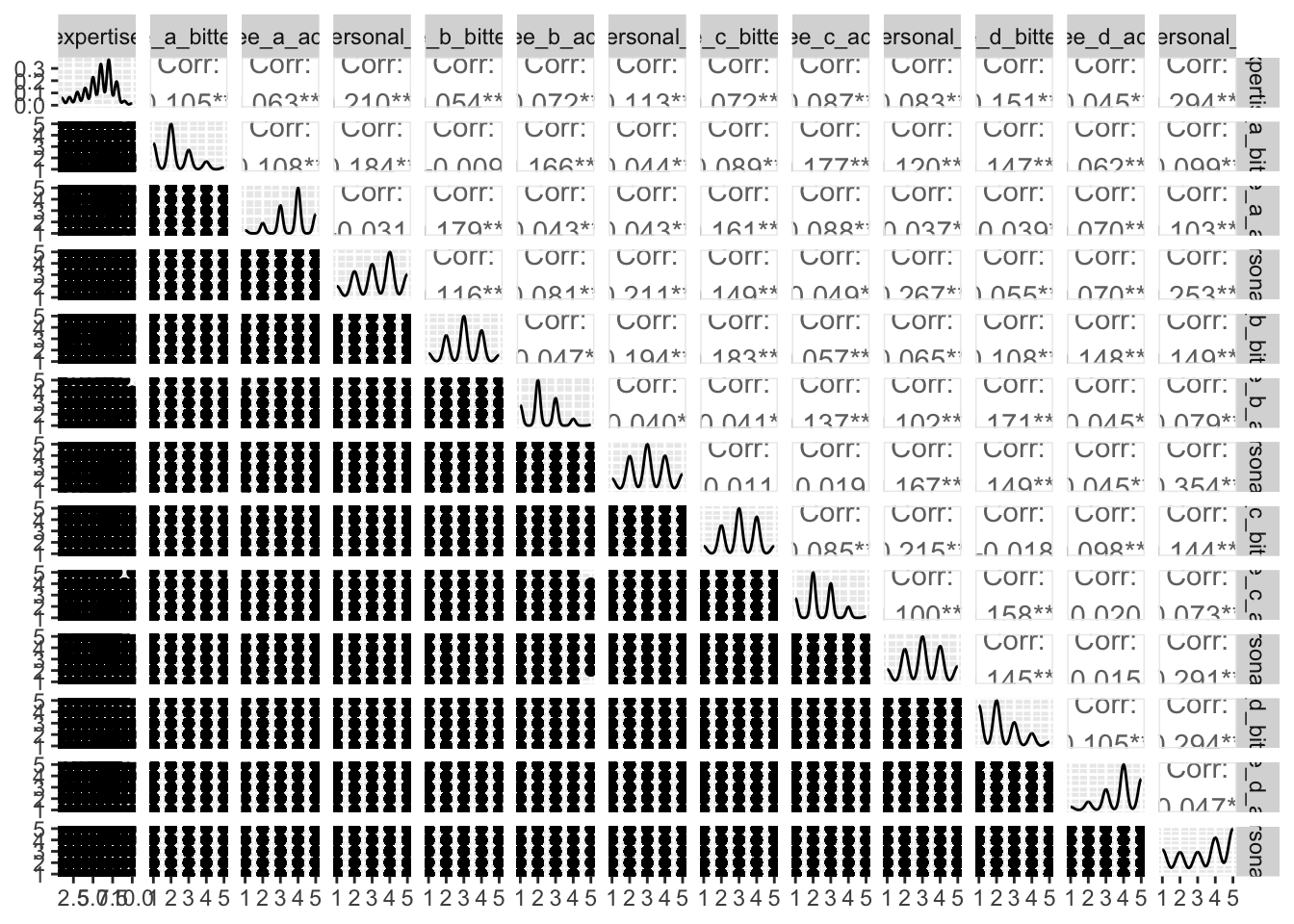
Demonstration: Generate a scatterplot matrix for all the numeric variables in the data set.1
1 Not particularly helpful for this dataset, but a good practice to get into.
Your turn: Examine the distribution of roast/gender and roast/cups. Describe the patterns you see and anything that is of particular interest given the model we will estimate.
# add code here# add code hereAdd response here.


