HW 03 - Tune and evaluate models

Homework

Modified

September 22, 2025

Important

This homework is due September 24 at 11:59pm ET.

Learning objectives

Tune and evaluate machine learning models
Implement methods for handling class imbalance
Select and interpret appropriate performance metrics

Getting started

Go to the info4940-fa25 organization on GitHub. Click on the repo with the prefix hw-03. It contains the starter documents you need to complete the lab.
Clone the repo and start a new workspace in Positron. See the Homework 0 instructions for details on cloning a repo and starting a new R project.

General guidance

Guidelines + tips

Set your random seed to ensure reproducible results.
Use caching to speed up the rendering process.
Use parallel processing to speed up rendering time. Note that this works differently on different systems and operating systems, and it also makes it harder to debug code and track progress in model fitting. Use at your own discretion.

Remember that continuing to develop a sound workflow for reproducible data analysis is important as you complete this homework and other assignments in this course. There will be periodic reminders in this assignment to remind you to render, commit, and push your changes to GitHub. You should have at least 3 commits with meaningful commit messages by the end of the assignment.

Workflow + formatting

Make sure to

Update author name on your document.
Label all code chunks informatively and concisely.
Follow consistent code style guidelines.
Make at least 3 commits.
Resize figures where needed, avoid tiny or huge plots.
Turn in an organized, well formatted document.

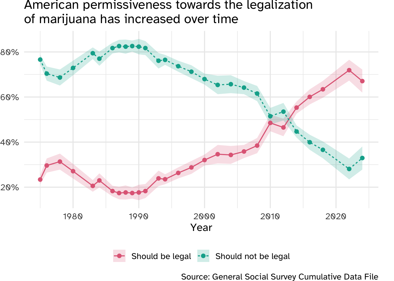
Attitudes towards marijuana legalization

The General Social Survey is a biannual survey of the American public.

Note

The GSS gathers data on contemporary American society in order to monitor and explain trends and constants in attitudes, behaviors, and attributes. Hundreds of trends have been tracked since 1972. In addition, since the GSS adopted questions from earlier surveys, trends can be followed for up to 70 years. The GSS contains a standard core of demographic, behavioral, and attitudinal questions, plus topics of special interest. Among the topics covered are civil liberties, crime and violence, intergroup tolerance, morality, national spending priorities, psychological well-being, social mobility, and stress and traumatic events.

Over the past 35 years, American attitudes towards marijuana have softened extensively. In the early 2010s, the number of Americans who believed marijuana should be legal began to outnumber those who thought it should not be legal.

data/gss.feather contains a selection of variables from the 2022 and 2024 GSS.¹ The outcome of interest grass is a variable coded as either "should be legal" (respondent believes marijuana should be legal) or "should not be legal" (respondent believes marijuana should not be legal).

Data summary
Name	gss
Number of rows	1591
Number of columns	25
_______________________
Column type frequency:
factor	21
numeric	4
________________________
Group variables	None

Variable type: factor

skim_variable	n_missing	complete_rate	ordered	n_unique	top_counts
colath	836	0.47	FALSE	2	yes: 473, not: 282
colmslm	841	0.47	FALSE	2	not: 546, yes: 204
degree	0	1.00	TRUE	5	hig: 793, bac: 282, les: 207, gra: 173
fear	818	0.49	FALSE	2	no: 503, yes: 270
grass	0	1.00	FALSE	2	sho: 1105, sho: 486
gunlaw	831	0.48	FALSE	2	fav: 517, opp: 243
happy	14	0.99	TRUE	3	pre: 854, not: 389, ver: 334
health	2	1.00	FALSE	4	goo: 767, fai: 449, exc: 262, poo: 111
hispanic	15	0.99	FALSE	5	not: 1332, mex: 116, ano: 78, pue: 33
income16	179	0.89	TRUE	26	$60: 128, $50: 117, $90: 109, $17: 102
letdie1	1211	0.24	FALSE	2	yes: 265, no: 115
owngun	812	0.49	FALSE	3	no: 507, yes: 245, ref: 27
partyid	22	0.99	TRUE	8	ind: 348, str: 261, not: 219, str: 197
polviews	99	0.94	TRUE	7	mod: 537, con: 222, sli: 199, sli: 194
pray	26	0.98	FALSE	6	sev: 587, onc: 349, nev: 238, sev: 164
pres20	538	0.66	FALSE	4	bid: 598, tru: 422, oth: 28, did: 5
race	33	0.98	FALSE	3	whi: 1012, bla: 355, oth: 191
region	0	1.00	FALSE	9	sou: 349, eas: 288, mid: 196, pac: 189
sex	2	1.00	FALSE	2	fem: 861, mal: 728
sexfreq	409	0.74	TRUE	7	not: 411, 2 o: 168, 2 o: 157, onc: 144
wrkstat	3	1.00	FALSE	8	wor: 602, ret: 438, kee: 171, wor: 150

Variable type: numeric

skim_variable	n_missing	complete_rate	mean	sd	p0	p25	p50	p75	p100	hist
id	0	1.00	992.85	572.81	2	501	973	1492.5	1990	▇▇▇▇▇
age	69	0.96	52.06	18.29	18	36	53	67.0	89	▆▇▆▇▃
hrs1	844	0.47	40.10	15.65	0	35	40	47.0	89	▁▂▇▂▁
wordsum	806	0.49	5.49	2.18	0	4	6	7.0	10	▂▅▇▅▂

What’s a feather file?

Feather is a portable file format for storing Arrow tables or data frames (from languages like Python or R) that utilizes the Arrow IPC format internally. Feather was created early in the Arrow project as a proof of concept for fast, language-agnostic data frame storage for Python (pandas) and R.

Essentially, it’s a fast binary format for storing tabular data that can be read and written quickly by multiple programming languages.

R
Python

library(arrow)

# Result is a tibble-formatted data frame
gss <- read_feather("data/gss.feather")

import pyarrow.feather as feather

# Result is pandas.DataFrame
gss = feather.read_feather("data/gss.feather")

Get detailed documentation for the variables

You can find the documentation for each of the available variables using the GSS Data Explorer. Just search by the column name to find the associated description.

Part 1 - Get familiar with the data

Exercise 1

Identify appropriate performance metrics. Select an appropriate set of performance metrics for evaluating classification models for predicting grass. Justify your choices.

Note

Use these metrics throughout the rest of the assignment except for exercises 4-5.

Difference between $J$-index and balanced accuracy

The $J$-index is defined as $\text{sensitivity} + \text{specificity} - 1$, while balanced accuracy is defined as $(\text{sensitivity} + \text{specificity}) / 2$. They are linearly related:

\[ \text{balanced accuracy} = \frac{\text{J-index} + 1}{2} \]

scikit-learn does not have a built-in metric for the $J$-index, but balanced accuracy is equivalent as a linear transformation. For the purposes of model evaluation and comparison, they can be used interchangeably.

Exercise 2

Import, partition, and explore the data. Import the data and reproducibly partition it into training and test sets. Briefly justify your choice of partitioning strategy. Conduct exploratory data analysis to understand the distributions of the outcome grass and some of the potential predictors. Summarize your findings.

Exercise 3

Resample the training data, fit a null model, and evaluate the results. Resample the training data using an appropriate method (justify your choice) and fit a null model to establish a baseline of comparison. Interpret the results of the null model.

Part 2 - Dealing with class imbalance

Hopefully one of the characteristics you noticed is that the majority of respondents favor legalization. This is a common issue in classification problems, known as class imbalance where one of the outcome classes dominates or is significantly larger than the other class(es).

One technique for handling this issue is to downsample the majority class. This involves randomly removing observations from the majority class until the class sizes achieve a desired ratio. But why would this be good? Isn’t this just throwing away data? Didn’t we learn that more is better?!?!?!

Exercise 4

Let’s evaluate these claims by comparing the performance of a model trained on the original data to one trained on a downsampled dataset.

You will fit two penalized regression models. Specifcally, you should estimate a Lasso regression model using all available variables (except id)² to predict grass and tune over the penalty tuning parameter. Required data preprocessing will include:

Impute all numeric predictors with the arithmetic mean
Normalize all numeric predictors to mean of 0 and variance of 1

For the downsampled model, you will downsample the majority class to achieve a 1:1 ratio of those in favor to those opposed.

How to implement downsampling

R
Python

Use an appropriate function from the {themis} package to downsample the majority class.

Use an appropriate function from the imbalanced-learn package to downsample the majority class. Do not simply use sklearn.utils.resample() to downsample the majority class. This is not a valid approach for handling class imbalance since the downsampling should be done as part of the model training process (e.g. within cross-validation folds) to avoid data leakage.

Tune both models using 10-fold cross-validation and at least 20 possible values for the penalty parameter. Estimate the models’ performance using sensitivity, specificity, ROC AUC, Brier class, and J-index.

Looking to learn more?

What happens if you vary the ratio used to downsample the dataset? How does this effect model performance?
In R, consider using workflow sets to streamline the process of fitting multiple models.

Exercise 5

If our goal is to identify both the positive and negative outcomes (e.g. squirrels and no squirrels), which approach is preferred: downsampling or not? Why?
If our goal is to identify both the positive and negative outcomes (e.g. squirrels and no squirrels), which metric should we use to finalize the model (i.e. select the appropriate penalty value)? Why?

Using metrics to select a final model

Remember that you do not have to always chose the model with the absolute largest or smallest value for a metric. Sometimes you are willing to trade-off performance for simplicity. See the select_*() functions from {tune} for other possible approaches.³

Part 3 - tune and evaluate models

Exercise 6

Fit a random forest model. Estimate a random forest model to predict grass as a function of all the other variables in the dataset (except id). Perform any required data preprocessing and explain why it is necessary. Implement feature engineering as you wish. Tune the model across relevant hyperparameters.⁴ How does this model perform?

Exercise 7

Fit a penalized logistic regression model. Estimate a penalized logistic regression model to predict grass. Incorporate appropriate data preprocessing steps to ensure the model is estimated correctly, as well as any feature engineering steps you think are appropriate to improve the model’s performance.

Tune the model across the penalty and mixture tuning parameters. If any feature engineering steps require tuning, include those as well.

Balanced grid tuning

If you are only tuning across penalty and mixture, I recommend a balanced grid tuning procedure. Because of how the penalty parameter is defined in a penalized regression model, you don’t need to estimate separate models for each value of penalty. You can estimate a single model for each value of mixture and then extract the coefficients for all values of penalty from that single model. This can significantly speed up the tuning process.

Implement a balanced grid tuning procedure. Interpret the results of the tuning procedure, including how the tuning parameters effect model performance as well as the overall performance of the “best” models.

Exercise 8

Choose your own adventure. Choose and fit a third model of your choice to predict grass. This can be any model you want, but it must be different from the random forest and penalized regression models you already fit. Document your choice of model and justify why you think it is appropriate for this problem. Perform any data preprocessing or feature engineering steps you think are appropriate to improve the model’s performance. Tune the model across relevant hyperparameters. How does this model perform?

Exercise 9

Pick the best performing model. Select the best performing model. Train that model using the full training set and report on it’s performance using the held-out test set of data. How would you describe this model’s performance at predicting attitudes towards the legalization of marijuana?

Bonus (optional) - Battle Royale

For those looking for a challenge (and a slight amount of extra credit for this assignment), train a high-performing model to predict grass.

To evaluate your model’s effectiveness, you will generate predictions for a held-back secret test set of respondents from the survey. These can be found in data/gss-test.rds. The data frame has an identical structure to gss.rds, however I have not included the grass column. You will have no way of judging the effectiveness of your model on the test set itself.

To evaluate your model’s performance, you must create a CSV file that contains your predicted probabilities for grass. This CSV should have three columns: id (the id value for the respondent), .pred_should be legal, and .pred_should not be legal. You can generate this CSV file using the code below:

R
Python

augment(best_fit, new_data = gss_secret_test) |>
  select(id, starts_with(".pred")) |>
  write_csv(file = "data/gss-preds.csv")

# Make predictions using your best model on the secret test set
predictions = best_model.predict_proba(X_secret_test)

# Create the results dataframe with the required format
results_df = pd.DataFrame({
    'id': gss_secret_test['id'],  # Extract ID from the secret test data
    '.pred_should be legal': predictions[:, 1],      # Probability of positive class
    '.pred_should not be legal': predictions[:, 0]   # Probability of negative class
})

# Save to CSV
results_df.to_csv("data/gss-preds.csv", index=False)

where gss_secret_test is a data frame imported from data/gss-test.rds and best_fit is the final model fitted using the entire training set.

Warning

Your CSV file must

Be structured exactly as I specified above.
Be stored in the data folder and named "gss-preds.csv".

If it does not meet these requirements, then you are not eligible to win this challenge.

The three students with the highest ROC AUC as calculated using their secret test set predictions will earn an extra (uncapped) 10 points on this homework assignment. For instance, if a student earned 45/50 points on the other components and was in the top-three, they would earn a 55/50 for this homework assignment.

Generative AI (GAI) self-reflection

As stated in the syllabus, include a written reflection for this assignment of how you used GAI tools (e.g. what tools you used, how you used them to assist you with writing code), what skills you believe you acquired, and how you believe you demonstrated mastery of the learning objectives.

Render, commit, and push one last time.

Make sure that you commit and push all changed documents and your Git pane is completely empty before proceeding.

Wrap up

Submission

Go to http://www.gradescope.com and click Log in in the top right corner.
Click School Credentials $\rightarrow$ Cornell University NetID and log in using your NetID credentials.
Click on your INFO 4940/5940 course.
Click on the assignment, and you’ll be prompted to submit it.
Mark all the pages associated with exercise. All the pages of your homework should be associated with at least one question (i.e., should be “checked”).

Grading

Exercise 1: 4 points
Exercise 2: 6 points
Exercise 3: 4 points
Exercise 4: 6 points
Exercise 5: 6 points
Exercise 6: 6 points
Exercise 7: 6 points
Exercise 8: 6 points
Exercise 9: 6 points
Bonus (optional): up to 10 extra points
GAI self-reflection: 0 points
Total: 50 points

Footnotes

For the purposes of this assignment, we will pool the observations and treat them as a single dataset.↩︎
Hopefully you figured it out by now, but do not use id for any of the models.↩︎
Sorry, I don’t know a great Python equivalent for this.↩︎
It’s up to you to decide which hyperparameters require tuning.↩︎