AE 11: Slay - Predicting song artist based on lyrics
Suggested answers
Import data
lyrics <- read_csv(file = "data/beyonce-swift-lyrics.csv") |>
  mutate(artist = factor(artist))
lyrics
# A tibble: 355 × 19
album_name track_number track_name artist lyrics danceability energy loudness
<chr> <dbl> <chr> <fct> <chr> <dbl> <dbl> <dbl>
1 COWBOY CA… 1 AMERIICAN… Beyon… "Noth… 0.374 0.515 -6.48
2 COWBOY CA… 3 16 CARRIA… Beyon… "Sixt… 0.525 0.456 -7.04
3 COWBOY CA… 5 MY ROSE Beyon… "How … 0.384 0.177 -11.8
4 COWBOY CA… 7 TEXAS HOL… Beyon… "This… 0.727 0.711 -6.55
5 COWBOY CA… 8 BODYGUARD Beyon… "One,… 0.726 0.779 -5.43
6 COWBOY CA… 10 JOLENE Beyon… "(Jol… 0.567 0.812 -5.43
7 COWBOY CA… 11 DAUGHTER Beyon… "Your… 0.374 0.448 -10.0
8 COWBOY CA… 13 ALLIIGATO… Beyon… "High… 0.618 0.651 -9.66
9 COWBOY CA… 18 FLAMENCO Beyon… "My m… 0.497 0.351 -9.25
10 COWBOY CA… 20 YA YA Beyon… "Hell… 0.617 0.904 -5.37
# ℹ 345 more rows
# ℹ 11 more variables: speechiness <dbl>, acousticness <dbl>,
# instrumentalness <dbl>, liveness <dbl>, valence <dbl>, tempo <dbl>,
# time_signature <dbl>, duration_ms <dbl>, explicit <lgl>, key_name <chr>,
# mode_name <chr>Split the data into analysis/assessment/test sets
Demonstration:
- Split the data into training/test sets with 75% allocated for training
- Split the training set into 10 cross-validation folds
# split into training/testing
set.seed(123)
lyrics_split <- initial_split(data = lyrics, strata = artist, prop = 0.75)

lyrics_train <- training(lyrics_split)
lyrics_test <- testing(lyrics_split)

# create cross-validation folds
lyrics_folds <- vfold_cv(data = lyrics_train, strata = artist)
Regularized regression
Define the feature engineering recipe
Demonstration:
- Define a feature engineering recipe to predict the song’s artist as a function of the lyrics + audio features
- Exclude the ID variables from the recipe
- Tokenize the song lyrics
- Calculate all possible 1-grams, 2-grams, 3-grams, 4-grams, and 5-grams
- Remove stop words
- Only keep the 2000 most frequently appearing tokens
- Calculate tf-idf scores for the remaining tokens
-
This will generate one column for every token. Each column will have the standardized name
tfidf_lyrics_*where*is the specific token. Instead we would prefer the column names simply be*. You can remove thetfidf_lyrics_prefix using# Simplify these names step_rename_at(starts_with("tfidf_lyrics_"), fn = \(x) str_replace_all( string = x, pattern = "tfidf_lyrics_", replacement = "" ) ) -
This does cause a conflict between the
energyaudio feature and the tokenenergy. Before removing the"tfidf_lyrics_"prefix, we will add a prefix to the audio features to avoid this conflict.# Simplify these names step_rename_at( all_predictors(), -starts_with("tfidf_lyrics_"), fn = \(x) str_glue("af_{x}") )
-
- Apply required steps for regularized regression models
- Convert the
explicitvariable to a factor - Convert nominal predictors to dummy variables
- Get rid of zero-variance predictors
- Normalize all predictors to mean of 0 and variance of 1
- Convert the
- Downsample the observations so there are an equal number of songs by Beyoncé and Taylor Swift in the analysis set
glmnet_rec <- recipe(artist ~ ., data = lyrics_train) |>
# exclude ID variables
update_role(album_name, track_number, track_name, new_role = "id vars") |>
# tokenize and prep lyrics
step_tokenize(lyrics) |>
step_stopwords(lyrics) |>
step_ngram(lyrics, num_tokens = 5L, min_num_tokens = 1L) |>
step_tokenfilter(lyrics, max_tokens = 4000) |>
step_tfidf(lyrics) |>
# Simplify these names
step_rename_at(
  all_predictors(), -starts_with("tfidf_lyrics_"),
  fn = \(x) str_glue("af_{x}")
) |>
step_rename_at(starts_with("tfidf_lyrics_"),
fn = \(x) str_replace_all(
string = x,
pattern = "tfidf_lyrics_",
replacement = ""
)
) |>
# fix explicit variable to factor
step_bin2factor(af_explicit) |>
# normalize for regularized regression
step_dummy(all_nominal_predictors()) |>
step_zv(all_predictors()) |>
step_normalize(all_numeric_predictors()) |>
step_downsample(artist)
glmnet_recWhat does this produce?
# A tibble: 176 × 4,028
   album_name    track_number track_name   af_danceability af_energy af_loudness
   <fct>                <dbl> <fct>                  <dbl>     <dbl>       <dbl>
 1 COWBOY CARTER            7 TEXAS HOLD …           1.10      0.782      0.478
 2 COWBOY CARTER            8 BODYGUARD              1.10      1.16       0.920
 3 COWBOY CARTER           10 JOLENE                -0.113     1.35       0.919
 4 COWBOY CARTER           11 DAUGHTER              -1.58     -0.689     -0.903
 5 COWBOY CARTER           13 ALLIIGATOR …           0.275     0.446     -0.753
 6 COWBOY CARTER           18 FLAMENCO              -0.646    -1.23      -0.589
 7 COWBOY CARTER           22 DESERT EAGLE           0.831    -0.459     -0.278
 8 COWBOY CARTER           23 RIIVERDANCE            0.892     1.23      -0.304
 9 COWBOY CARTER           24 II HANDS II…           0.701     0.172     -0.0427
10 COWBOY CARTER           27 AMEN                  -1.89     -0.666      0.266
# ℹ 166 more rows
# ℹ 4,022 more variables: af_speechiness <dbl>, af_acousticness <dbl>,
#   af_instrumentalness <dbl>, af_liveness <dbl>, af_valence <dbl>,
#   af_tempo <dbl>, af_time_signature <dbl>, af_duration_ms <dbl>,
#   artist <fct>, `1` <dbl>, `2` <dbl>, `3` <dbl>, `4` <dbl>, across <dbl>,
#   act <dbl>, actin <dbl>, acting <dbl>, actress <dbl>, adore <dbl>,
#   adore_adore <dbl>, adore_adore_adore <dbl>, affair <dbl>, afraid <dbl>, …
Tune the regularized regression model
Demonstration:
- Define the regularized regression model specification, including tuning placeholders for
penalty - Create the workflow object
- Define a tuning grid over
penalty - Tune the model using the cross-validation folds
- Evaluate the tuning procedure and identify the best performing models based on ROC AUC
# define the regularized regression model specification
glmnet_spec <- logistic_reg(penalty = tune(), mixture = 1) |>
  set_mode("classification") |>
  set_engine("glmnet")

# define the new workflow
glmnet_wf <- workflow() |>
  add_recipe(glmnet_rec) |>
  add_model(glmnet_spec)

# create the tuning grid
glmnet_grid <- grid_regular(
  penalty(),
  levels = 30
)

# tune over the model hyperparameters
glmnet_tune <- tune_grid(
  object = glmnet_wf,
  resamples = lyrics_folds,
  grid = glmnet_grid,
  control = control_grid(save_workflow = TRUE)
)
# evaluate results
autoplot(glmnet_tune)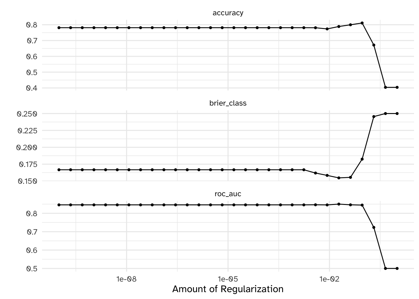
# identify the five best hyperparameter combinations
show_best(x = glmnet_tune, metric = "roc_auc")
# A tibble: 5 × 7
penalty .metric .estimator mean n std_err .config
<dbl> <chr> <chr> <dbl> <int> <dbl> <chr>
1 1.89e- 2 roc_auc binary 0.850 10 0.0260 Preprocessor1_Model25
2 3.86e- 3 roc_auc binary 0.846 10 0.0260 Preprocessor1_Model23
3 4.18e- 2 roc_auc binary 0.846 10 0.0264 Preprocessor1_Model26
4 1 e-10 roc_auc binary 0.846 10 0.0262 Preprocessor1_Model01
5 2.21e-10 roc_auc binary 0.846 10 0.0262 Preprocessor1_Model02Variable importance
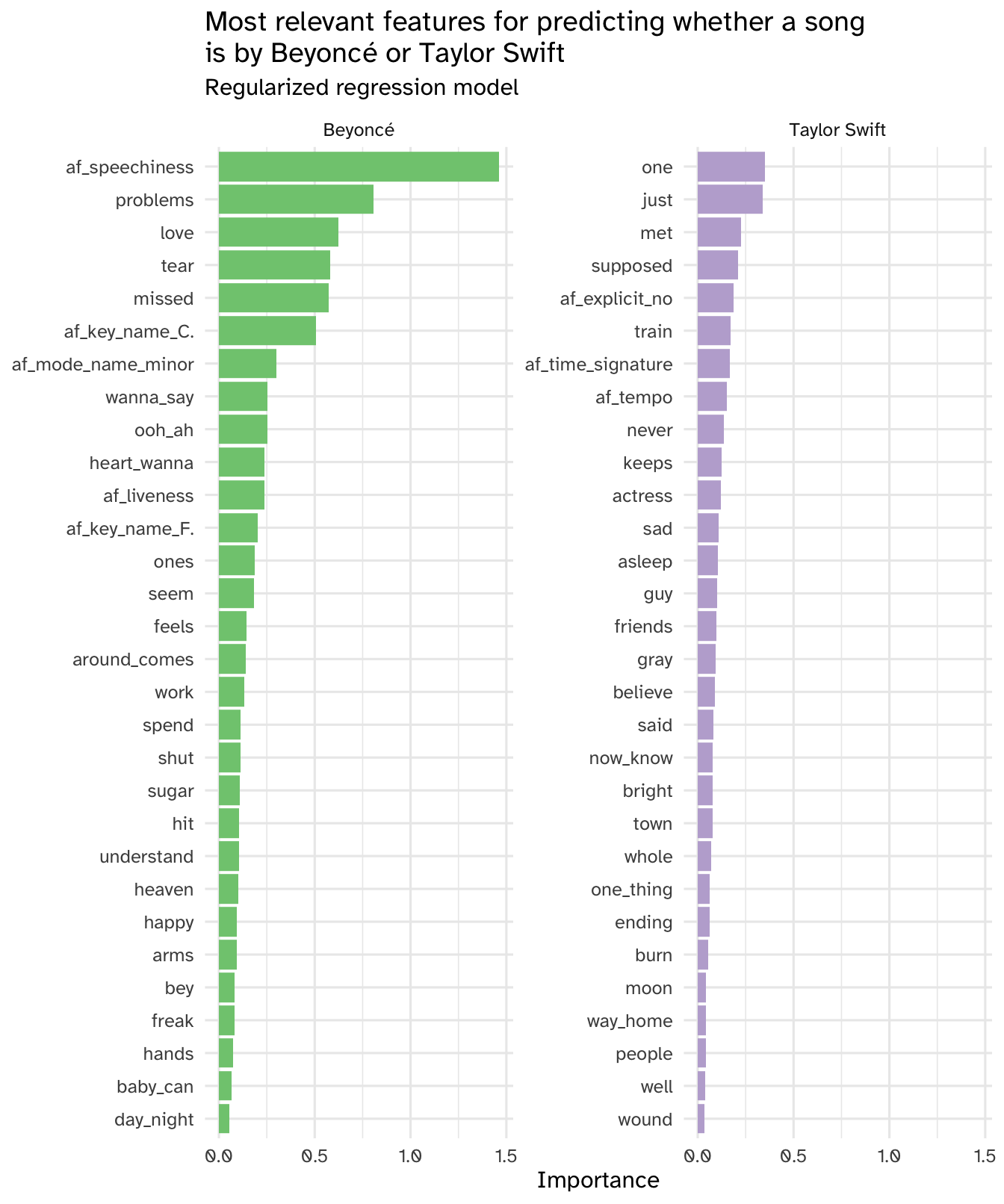
Your turn: Identify the most relevant features for predicting whether a song is by Beyoncé or Taylor Swift using the regularized regression model. How many features are used in the final model?
# extract parsnip model fit
glmnet_imp <- glmnet_tune |>
  fit_best() |>
  extract_fit_parsnip() |>
  vi(method = "model", lambda = select_best(x = glmnet_tune, metric = "roc_auc")$penalty)

# top features
vip(glmnet_imp)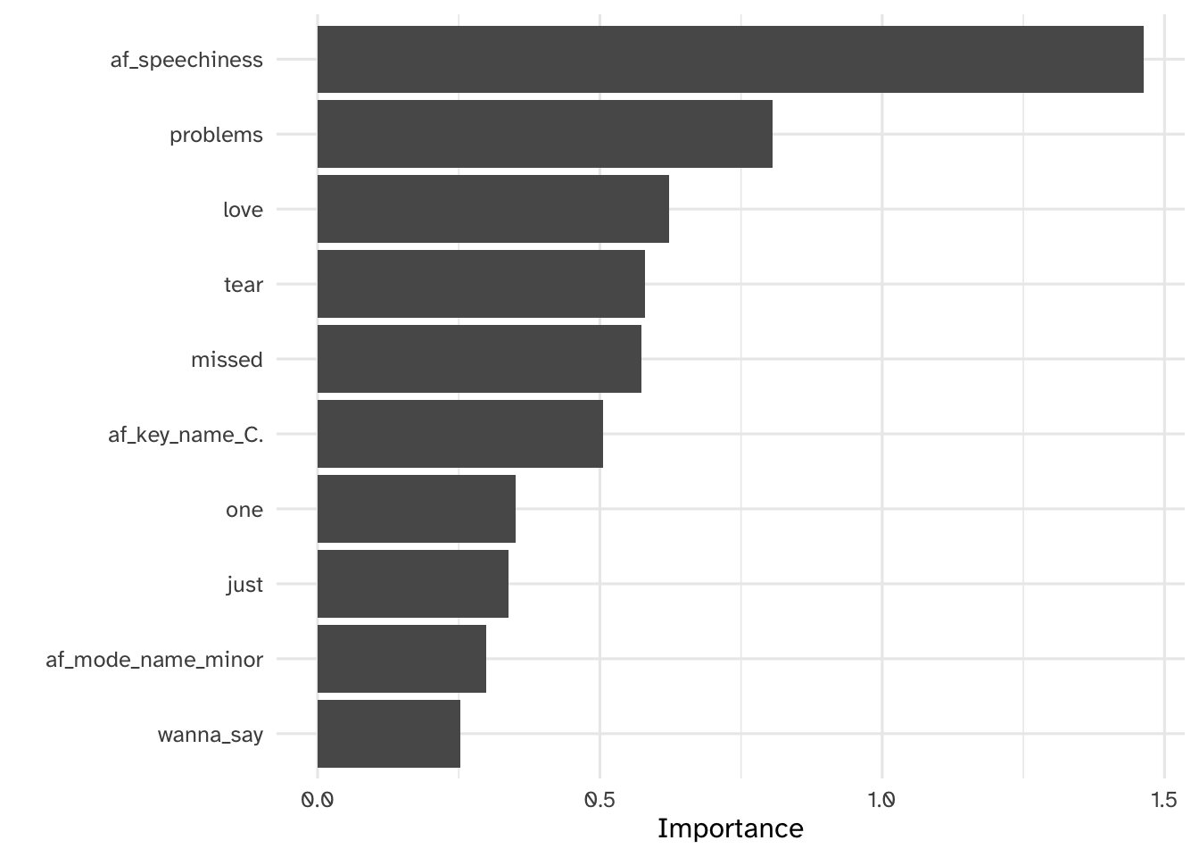
# features with non-zero coefficients
glmnet_imp |>
  # importance must be greater than 0
  filter(Importance > 0)
# A tibble: 108 × 3
Variable Importance Sign
<chr> <dbl> <chr>
1 af_speechiness 1.46 NEG
2 problems 0.806 NEG
3 love 0.623 NEG
4 tear 0.580 NEG
5 missed 0.574 NEG
6 af_key_name_C. 0.506 NEG
7 one 0.350 POS
8 just 0.338 POS
9 af_mode_name_minor 0.299 NEG
10 wanna_say 0.252 NEG
# ℹ 98 more rowsAdd response here. The final model used only 108 features, a substantial reduction from the original number.
Your turn: Interpret the most relevant features for predicting whether a song is by Beyoncé or Taylor Swift. As a gut check, do these results make sense to you based on your knowledge of these artists?
# clean up the data frame for visualization
glmnet_imp |>
  # because Taylor Swift is labeled the "success" outcome,
  # positive coefficients indicate higher probability of being a Taylor Swift song
  mutate(Sign = if_else(Sign == "POS", "Taylor Swift", "Beyoncé")) |>
  # importance must be greater than 0
  filter(Importance > 0) |>
  # keep top 30 features for each artist
  slice_max(n = 30, order_by = Importance, by = Sign) |>
  mutate(Variable = fct_reorder(.f = Variable, .x = Importance)) |>
  ggplot(mapping = aes(
    x = Importance,
    y = Variable,
    fill = Sign
  )) +
  geom_col(show.legend = FALSE) +
  scale_fill_brewer(type = "qual") +
  facet_wrap(facets = vars(Sign), scales = "free_y") +
  labs(
    y = NULL,
    title = "Most relevant features for predicting whether a song\nis by Beyoncé or Taylor Swift",
    subtitle = "Regularized regression model"
  )
Add response here. Sort of based on my naive and biased understandings of the two artists. The audio features seem more understandable as opposed to specific song lyrics, but again I am not part of the Beyhive nor a Swiftie.
Fit a random forest model
Define the feature engineering recipe
Demonstration:
- Define a feature engineering recipe to predict the song’s artist as a function of the lyrics + audio features
- Exclude the ID variables from the recipe
- Tokenize the song lyrics
- Remove stop words
- Only keep the 500 most frequently appearing tokens
- Calculate tf-idf scores for the remaining tokens
- Rename audio feature and tf-idf as before
- Downsample the observations so there are an equal number of songs by Beyoncé and Taylor Swift in the analysis set
# define preprocessing recipe
rf_rec <- recipe(artist ~ ., data = lyrics_train) |>
  # exclude ID variables
  update_role(album_name, track_number, track_name, new_role = "id vars") |>
  step_tokenize(lyrics) |>
  step_stopwords(lyrics) |>
  step_tokenfilter(lyrics, max_tokens = 500) |>
  step_tfidf(lyrics) |>
  # Simplify these names
  step_rename_at(
    all_predictors(), -starts_with("tfidf_lyrics_"),
    fn = \(x) str_glue("af_{x}")
  ) |>
  step_rename_at(starts_with("tfidf_lyrics_"),
    fn = \(x) str_replace_all(
      string = x,
      pattern = "tfidf_lyrics_",
      replacement = ""
    )
  ) |>
  step_downsample(artist)
rf_rec
What does this produce?
# A tibble: 176 × 518
   album_name    track_number track_name   af_danceability af_energy af_loudness
   <fct>                <dbl> <fct>                  <dbl>     <dbl>       <dbl>
 1 COWBOY CARTER            7 TEXAS HOLD …           0.727     0.711       -6.55
 2 COWBOY CARTER            8 BODYGUARD              0.726     0.779       -5.43
 3 COWBOY CARTER           10 JOLENE                 0.567     0.812       -5.43
 4 COWBOY CARTER           11 DAUGHTER               0.374     0.448      -10.0
 5 COWBOY CARTER           13 ALLIIGATOR …           0.618     0.651       -9.66
 6 COWBOY CARTER           18 FLAMENCO               0.497     0.351       -9.25
 7 COWBOY CARTER           22 DESERT EAGLE           0.691     0.489       -8.46
 8 COWBOY CARTER           23 RIIVERDANCE            0.699     0.791       -8.53
 9 COWBOY CARTER           24 II HANDS II…           0.674     0.602       -7.87
10 COWBOY CARTER           27 AMEN                   0.333     0.452       -7.09
# ℹ 166 more rows
# ℹ 512 more variables: af_speechiness <dbl>, af_acousticness <dbl>,
#   af_instrumentalness <dbl>, af_liveness <dbl>, af_valence <dbl>,
#   af_tempo <dbl>, af_time_signature <dbl>, af_duration_ms <dbl>,
#   af_explicit <lgl>, af_key_name <fct>, af_mode_name <fct>, artist <fct>,
#   adore <dbl>, afraid <dbl>, ah <dbl>, `ain't` <dbl>, air <dbl>, alive <dbl>,
#   almost <dbl>, alone <dbl>, along <dbl>, alright <dbl>, always <dbl>, …
Fit the model
Demonstration:
- Define a random forest model grown with 1000 trees using the
rangerengine. - Define a workflow using the feature engineering recipe and random forest model specification. Fit the workflow using the entire training set (no cross-validation necessary).
# define the model specification
rf_spec <- rand_forest(trees = 1000) |>
  set_mode("classification") |>
  # calculate feature importance metrics using the ranger engine
  set_engine("ranger", importance = "permutation")

# define the workflow
rf_wf <- workflow() |>
  add_recipe(rf_rec) |>
  add_model(rf_spec)

# fit the model to the training set
rf_fit <- rf_wf |>
  fit(data = lyrics_train)
Feature importance
Your turn: Interpret the most relevant features for predicting whether a song is by Beyoncé or Taylor Swift using the random forest approach. As a gut check, do these results make sense to you based on your knowledge of these artists? How do they compare to the results from regularized regression?
# extract parsnip model fit
rf_imp <- rf_fit |>
  extract_fit_parsnip() |>
  vi(method = "model")

# naive attempt to interpret
vip(rf_imp)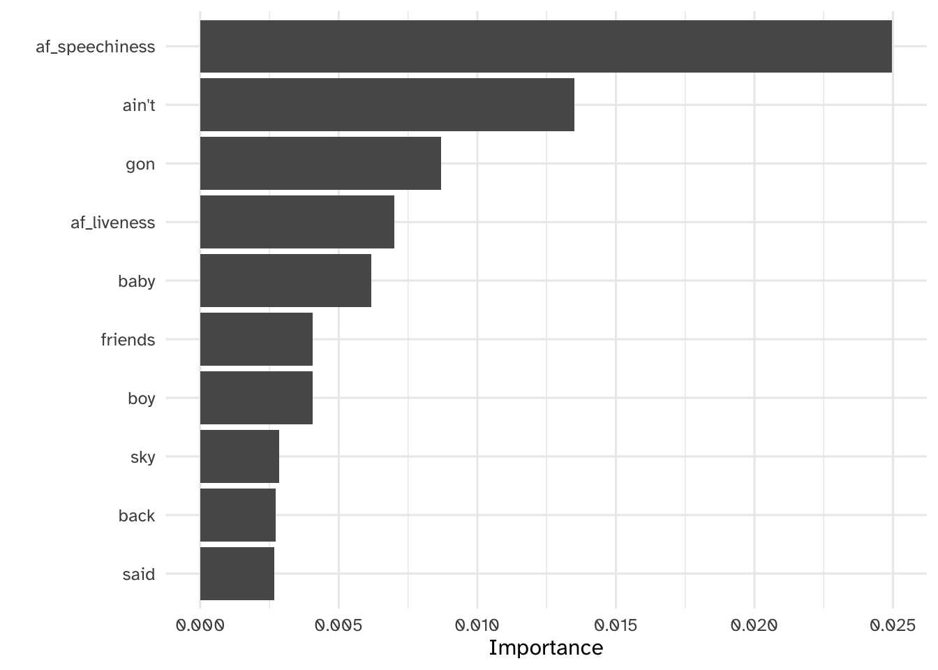
# clean up the data frame for visualization
rf_imp |>
  # extract 30 most important n-grams
  slice_max(order_by = Importance, n = 30) |>
  mutate(Variable = fct_reorder(.f = Variable, .x = Importance)) |>
  ggplot(mapping = aes(
    x = Importance,
    y = Variable
  )) +
  geom_col() +
  scale_x_continuous(labels = label_percent()) +
  labs(
    x = "Increase in OOB error rate",
    y = NULL,
    title = "Most relevant features for predicting whether a song\nis by Beyoncé or Taylor Swift",
    subtitle = "Random forest model"
  )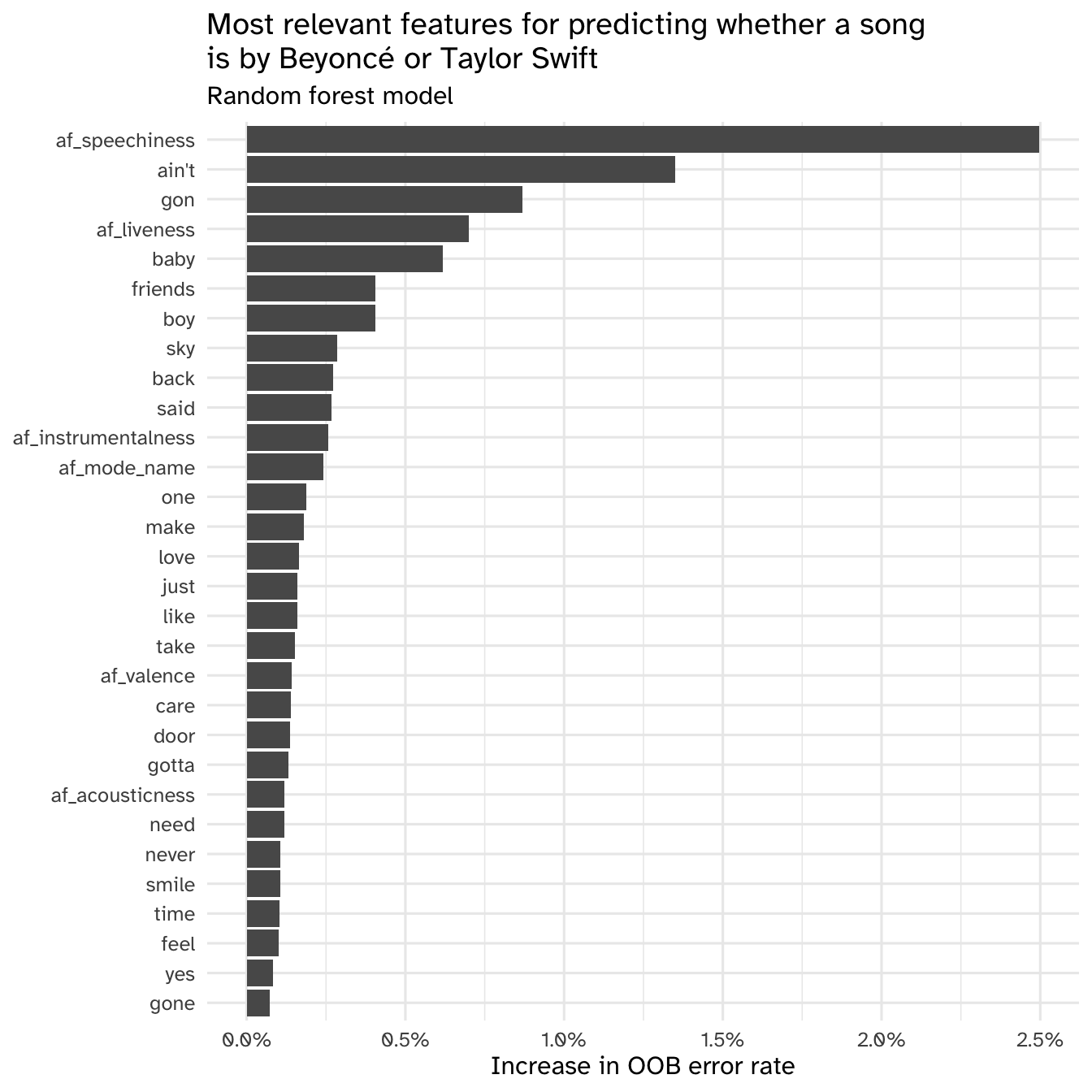
Add response here. The random forest model identified some of the same features as the lasso regression (speechiness, song modality) but a lot of the lyrics seem to differ. This is potentially driven by the different tokenization techniques for each model (random forest only had unigrams, whereas the lasso regression had up to 5-grams).
sessioninfo::session_info()─ Session info ───────────────────────────────────────────────────────────────
setting value
version R version 4.4.1 (2024-06-14)
os macOS Sonoma 14.6.1
system aarch64, darwin20
ui X11
language (EN)
collate en_US.UTF-8
ctype en_US.UTF-8
tz America/New_York
date 2024-10-10
pandoc 3.4 @ /usr/local/bin/ (via rmarkdown)
─ Packages ───────────────────────────────────────────────────────────────────
package * version date (UTC) lib source
archive 1.1.8 2024-04-28 [1] CRAN (R 4.4.0)
backports 1.5.0 2024-05-23 [1] CRAN (R 4.4.0)
bit 4.0.5 2022-11-15 [1] CRAN (R 4.3.0)
bit64 4.0.5 2020-08-30 [1] CRAN (R 4.3.0)
broom * 1.0.6 2024-05-17 [1] CRAN (R 4.4.0)
class 7.3-22 2023-05-03 [1] CRAN (R 4.4.0)
cli 3.6.3 2024-06-21 [1] CRAN (R 4.4.0)
codetools 0.2-20 2024-03-31 [1] CRAN (R 4.4.1)
colorspace 2.1-1 2024-07-26 [1] CRAN (R 4.4.0)
crayon 1.5.3 2024-06-20 [1] CRAN (R 4.4.0)
data.table 1.15.4 2024-03-30 [1] CRAN (R 4.3.1)
dials * 1.3.0 2024-07-30 [1] CRAN (R 4.4.0)
DiceDesign 1.10 2023-12-07 [1] CRAN (R 4.3.1)
digest 0.6.35 2024-03-11 [1] CRAN (R 4.3.1)
discrim * 1.0.1 2023-03-08 [1] CRAN (R 4.4.0)
dplyr * 1.1.4 2023-11-17 [1] CRAN (R 4.3.1)
ellipsis 0.3.2 2021-04-29 [1] CRAN (R 4.3.0)
evaluate 0.24.0 2024-06-10 [1] CRAN (R 4.4.0)
fansi 1.0.6 2023-12-08 [1] CRAN (R 4.3.1)
farver 2.1.2 2024-05-13 [1] CRAN (R 4.3.3)
fastmap 1.2.0 2024-05-15 [1] CRAN (R 4.4.0)
forcats * 1.0.0 2023-01-29 [1] CRAN (R 4.3.0)
foreach 1.5.2 2022-02-02 [1] CRAN (R 4.3.0)
fs 1.6.4 2024-04-25 [1] CRAN (R 4.4.0)
furrr 0.3.1 2022-08-15 [1] CRAN (R 4.3.0)
future 1.33.2 2024-03-26 [1] CRAN (R 4.3.1)
future.apply 1.11.2 2024-03-28 [1] CRAN (R 4.3.1)
generics 0.1.3 2022-07-05 [1] CRAN (R 4.3.0)
ggplot2 * 3.5.1 2024-04-23 [1] CRAN (R 4.3.1)
glmnet * 4.1-8 2023-08-22 [1] CRAN (R 4.3.0)
globals 0.16.3 2024-03-08 [1] CRAN (R 4.3.1)
glue 1.8.0 2024-09-30 [1] CRAN (R 4.4.1)
gower 1.0.1 2022-12-22 [1] CRAN (R 4.3.0)
GPfit 1.0-8 2019-02-08 [1] CRAN (R 4.3.0)
gtable 0.3.5 2024-04-22 [1] CRAN (R 4.3.1)
hardhat 1.4.0 2024-06-02 [1] CRAN (R 4.4.0)
here 1.0.1 2020-12-13 [1] CRAN (R 4.3.0)
hms 1.1.3 2023-03-21 [1] CRAN (R 4.3.0)
htmltools 0.5.8.1 2024-04-04 [1] CRAN (R 4.3.1)
htmlwidgets 1.6.4 2023-12-06 [1] CRAN (R 4.3.1)
infer * 1.0.7 2024-03-25 [1] CRAN (R 4.3.1)
ipred 0.9-14 2023-03-09 [1] CRAN (R 4.3.0)
iterators 1.0.14 2022-02-05 [1] CRAN (R 4.3.0)
jsonlite 1.8.9 2024-09-20 [1] CRAN (R 4.4.1)
knitr 1.47 2024-05-29 [1] CRAN (R 4.4.0)
labeling 0.4.3 2023-08-29 [1] CRAN (R 4.3.0)
lattice 0.22-6 2024-03-20 [1] CRAN (R 4.4.0)
lava 1.8.0 2024-03-05 [1] CRAN (R 4.3.1)
lhs 1.1.6 2022-12-17 [1] CRAN (R 4.3.0)
lifecycle 1.0.4 2023-11-07 [1] CRAN (R 4.3.1)
listenv 0.9.1 2024-01-29 [1] CRAN (R 4.3.1)
lubridate * 1.9.3 2023-09-27 [1] CRAN (R 4.3.1)
magrittr 2.0.3 2022-03-30 [1] CRAN (R 4.3.0)
MASS 7.3-61 2024-06-13 [1] CRAN (R 4.4.0)
Matrix * 1.7-0 2024-03-22 [1] CRAN (R 4.4.0)
modeldata * 1.4.0 2024-06-19 [1] CRAN (R 4.4.0)
munsell 0.5.1 2024-04-01 [1] CRAN (R 4.3.1)
nnet 7.3-19 2023-05-03 [1] CRAN (R 4.4.0)
parallelly 1.37.1 2024-02-29 [1] CRAN (R 4.3.1)
parsnip * 1.2.1 2024-03-22 [1] CRAN (R 4.3.1)
pillar 1.9.0 2023-03-22 [1] CRAN (R 4.3.0)
pkgconfig 2.0.3 2019-09-22 [1] CRAN (R 4.3.0)
prodlim 2023.08.28 2023-08-28 [1] CRAN (R 4.3.0)
purrr * 1.0.2 2023-08-10 [1] CRAN (R 4.3.0)
R6 2.5.1 2021-08-19 [1] CRAN (R 4.3.0)
ranger 0.16.0 2023-11-12 [1] CRAN (R 4.3.1)
RColorBrewer 1.1-3 2022-04-03 [1] CRAN (R 4.3.0)
Rcpp 1.0.13 2024-07-17 [1] CRAN (R 4.4.0)
readr * 2.1.5 2024-01-10 [1] CRAN (R 4.3.1)
recipes * 1.0.10 2024-02-18 [1] CRAN (R 4.3.1)
rlang 1.1.4 2024-06-04 [1] CRAN (R 4.3.3)
rmarkdown 2.27 2024-05-17 [1] CRAN (R 4.4.0)
ROSE 0.0-4 2021-06-14 [1] CRAN (R 4.3.0)
rpart 4.1.23 2023-12-05 [1] CRAN (R 4.4.0)
rprojroot 2.0.4 2023-11-05 [1] CRAN (R 4.3.1)
rsample * 1.2.1 2024-03-25 [1] CRAN (R 4.3.1)
rstudioapi 0.16.0 2024-03-24 [1] CRAN (R 4.3.1)
scales * 1.3.0 2023-11-28 [1] CRAN (R 4.4.0)
sessioninfo 1.2.2 2021-12-06 [1] CRAN (R 4.3.0)
shape 1.4.6.1 2024-02-23 [1] CRAN (R 4.3.1)
SnowballC 0.7.1 2023-04-25 [1] CRAN (R 4.3.0)
stopwords * 2.3 2021-10-28 [1] CRAN (R 4.3.0)
stringi 1.8.4 2024-05-06 [1] CRAN (R 4.3.1)
stringr * 1.5.1 2023-11-14 [1] CRAN (R 4.3.1)
survival 3.7-0 2024-06-05 [1] CRAN (R 4.4.0)
textdata * 0.4.5 2024-05-28 [1] CRAN (R 4.4.0)
textrecipes * 1.0.6 2023-11-15 [1] CRAN (R 4.3.1)
themis * 1.0.2 2023-08-14 [1] CRAN (R 4.3.0)
tibble * 3.2.1 2023-03-20 [1] CRAN (R 4.3.0)
tidymodels * 1.2.0 2024-03-25 [1] CRAN (R 4.3.1)
tidyr * 1.3.1 2024-01-24 [1] CRAN (R 4.3.1)
tidyselect 1.2.1 2024-03-11 [1] CRAN (R 4.3.1)
tidyverse * 2.0.0 2023-02-22 [1] CRAN (R 4.3.0)
timechange 0.3.0 2024-01-18 [1] CRAN (R 4.3.1)
timeDate 4032.109 2023-12-14 [1] CRAN (R 4.3.1)
tokenizers 0.3.0 2022-12-22 [1] CRAN (R 4.3.0)
tune * 1.2.1 2024-04-18 [1] CRAN (R 4.3.1)
tzdb 0.4.0 2023-05-12 [1] CRAN (R 4.3.0)
utf8 1.2.4 2023-10-22 [1] CRAN (R 4.3.1)
vctrs 0.6.5 2023-12-01 [1] CRAN (R 4.3.1)
vip * 0.4.1 2023-08-21 [1] CRAN (R 4.3.0)
vroom 1.6.5 2023-12-05 [1] CRAN (R 4.3.1)
withr 3.0.1 2024-07-31 [1] CRAN (R 4.4.0)
workflows * 1.1.4 2024-02-19 [1] CRAN (R 4.3.1)
workflowsets * 1.1.0 2024-03-21 [1] CRAN (R 4.3.1)
xfun 0.45 2024-06-16 [1] CRAN (R 4.4.0)
yaml 2.3.10 2024-07-26 [1] CRAN (R 4.4.0)
yardstick * 1.3.1 2024-03-21 [1] CRAN (R 4.3.1)
[1] /Library/Frameworks/R.framework/Versions/4.4-arm64/Resources/library
──────────────────────────────────────────────────────────────────────────────