library(tidyverse)
library(tidymodels)
library(colorspace)
library(skimr)
library(GGally)

set.seed(167)

# preferred theme
theme_set(theme_minimal(base_size = 12, base_family = "Atkinson Hyperlegible"))AE 09: Explore coffee taste tests
Suggested answers
Application exercise
Answers
R
Python
The Great American Coffee Taste Test
import pandas as pd
import numpy as np
from plotnine import *
from skimpy import skim
from sklearn.model_selection import train_test_split

# Set random seed
np.random.seed(167)

# Set preferred theme
theme_set(theme_minimal(base_size=12, base_family="Atkinson Hyperlegible"))
In October 2023, James Hoffmann and coffee company Cometeer held the “Great American Coffee Taste Test” on YouTube, during which viewers were asked to fill out a survey about 4 coffees they ordered from Cometeer for the tasting. Tidy Tuesday published the data set we are using.
coffee_survey <- read_csv(file = "data/coffee_survey.csv")

# partition into training and test sets
coffee_split <- initial_split(coffee_survey, prop = 0.8)
coffee_train <- training(coffee_split)
coffee_test <- testing(coffee_split)
coffee_survey = pd.read_csv("data/coffee_survey.csv")
# partition into training and test sets
coffee_train, coffee_test = train_test_split(coffee_survey, test_size=0.2, random_state=167)It includes the following features:
| variable | class | description |
|---|---|---|
| submission_id | character | Submission ID |
| age | character | What is your age? |
| cups | character | How many cups of coffee do you typically drink per day? |
| where_drink | character | Where do you typically drink coffee? |
| brew | character | How do you brew coffee at home? |
| brew_other | character | How else do you brew coffee at home? |
| purchase | character | On the go, where do you typically purchase coffee? |
| purchase_other | character | Where else do you purchase coffee? |
| favorite | character | What is your favorite coffee drink? |
| favorite_specify | character | Please specify what your favorite coffee drink is |
| additions | character | Do you usually add anything to your coffee? |
| additions_other | character | What else do you add to your coffee? |
| dairy | character | What kind of dairy do you add? |
| sweetener | character | What kind of sugar or sweetener do you add? |
| style | character | Before today’s tasting, which of the following best described what kind of coffee you like? |
| strength | character | How strong do you like your coffee? |
| roast_level | character | What roast level of coffee do you prefer? |
| caffeine | character | How much caffeine do you like in your coffee? |
| expertise | numeric | Lastly, how would you rate your own coffee expertise? |
| coffee_a_bitterness | numeric | Coffee A - Bitterness |
| coffee_a_acidity | numeric | Coffee A - Acidity |
| coffee_a_personal_preference | numeric | Coffee A - Personal Preference |
| coffee_a_notes | character | Coffee A - Notes |
| coffee_b_bitterness | numeric | Coffee B - Bitterness |
| coffee_b_acidity | numeric | Coffee B - Acidity |
| coffee_b_personal_preference | numeric | Coffee B - Personal Preference |
| coffee_b_notes | character | Coffee B - Notes |
| coffee_c_bitterness | numeric | Coffee C - Bitterness |
| coffee_c_acidity | numeric | Coffee C - Acidity |
| coffee_c_personal_preference | numeric | Coffee C - Personal Preference |
| coffee_c_notes | character | Coffee C - Notes |
| coffee_d_bitterness | numeric | Coffee D - Bitterness |
| coffee_d_acidity | numeric | Coffee D - Acidity |
| coffee_d_personal_preference | numeric | Coffee D - Personal Preference |
| coffee_d_notes | character | Coffee D - Notes |
| prefer_abc | character | Between Coffee A, Coffee B, and Coffee C which did you prefer? |
| prefer_ad | character | Between Coffee A and Coffee D, which did you prefer? |
| prefer_overall | character | Lastly, what was your favorite overall coffee? |
| wfh | character | Do you work from home or in person? |
| total_spend | character | In total, much money do you typically spend on coffee in a month? |
| why_drink | character | Why do you drink coffee? |
| why_drink_other | character | Other reason for drinking coffee |
| taste | character | Do you like the taste of coffee? |
| know_source | character | Do you know where your coffee comes from? |
| most_paid | character | What is the most you’ve ever paid for a cup of coffee? |
| most_willing | character | What is the most you’d ever be willing to pay for a cup of coffee? |
| value_cafe | character | Do you feel like you’re getting good value for your money when you buy coffee at a cafe? |
| spent_equipment | character | Approximately how much have you spent on coffee equipment in the past 5 years? |
| value_equipment | character | Do you feel like you’re getting good value for your money when you buy coffee at a cafe? |
| gender | character | Gender |
| gender_specify | character | Gender (please specify) |
| education_level | character | Education Level |
| ethnicity_race | character | Ethnicity/Race |
| ethnicity_race_specify | character | Ethnicity/Race (please specify) |
| employment_status | character | Employment Status |
| number_children | character | Number of Children |
| political_affiliation | character | Political Affiliation |
Our ultimate goal on a future assignment is to predict whether or not individuals like coffee D based on their survey responses and taste tests for coffees A-C.1 We will use a binary form of coffee_d_personal_preference variable as our target.
A quick skim of the data:
skim(coffee_train)| Name | coffee_train |
| Number of rows | 3233 |
| Number of columns | 57 |
| _______________________ | |
| Column type frequency: | |
| character | 44 |
| numeric | 13 |
| ________________________ | |
| Group variables | None |
Variable type: character
| skim_variable | n_missing | complete_rate | min | max | empty | n_unique | whitespace |
|---|---|---|---|---|---|---|---|
| submission_id | 0 | 1.00 | 6 | 6 | 0 | 3233 | 0 |
| age | 26 | 0.99 | 13 | 15 | 0 | 7 | 0 |
| cups | 79 | 0.98 | 1 | 11 | 0 | 6 | 0 |
| where_drink | 60 | 0.98 | 7 | 44 | 0 | 64 | 0 |
| brew | 320 | 0.90 | 5 | 165 | 0 | 401 | 0 |
| brew_other | 2687 | 0.17 | 2 | 105 | 0 | 130 | 0 |
| purchase | 2659 | 0.18 | 5 | 107 | 0 | 77 | 0 |
| purchase_other | 3214 | 0.01 | 4 | 83 | 0 | 16 | 0 |
| favorite | 55 | 0.98 | 5 | 32 | 0 | 12 | 0 |
| favorite_specify | 3145 | 0.03 | 3 | 64 | 0 | 62 | 0 |
| additions | 71 | 0.98 | 5 | 100 | 0 | 47 | 0 |
| additions_other | 3194 | 0.01 | 3 | 140 | 0 | 34 | 0 |
| dairy | 1876 | 0.42 | 8 | 110 | 0 | 148 | 0 |
| sweetener | 2821 | 0.13 | 5 | 99 | 0 | 77 | 0 |
| style | 71 | 0.98 | 4 | 11 | 0 | 12 | 0 |
| strength | 102 | 0.97 | 4 | 15 | 0 | 5 | 0 |
| roast_level | 84 | 0.97 | 4 | 7 | 0 | 7 | 0 |
| caffeine | 103 | 0.97 | 5 | 13 | 0 | 3 | 0 |
| coffee_a_notes | 1166 | 0.64 | 3 | 377 | 0 | 1863 | 0 |
| coffee_b_notes | 1265 | 0.61 | 1 | 980 | 0 | 1781 | 0 |
| coffee_c_notes | 1319 | 0.59 | 2 | 438 | 0 | 1749 | 0 |
| coffee_d_notes | 1159 | 0.64 | 2 | 528 | 0 | 1903 | 0 |
| prefer_abc | 215 | 0.93 | 8 | 8 | 0 | 3 | 0 |
| prefer_ad | 223 | 0.93 | 8 | 8 | 0 | 2 | 0 |
| prefer_overall | 216 | 0.93 | 8 | 8 | 0 | 4 | 0 |
| wfh | 417 | 0.87 | 18 | 26 | 0 | 3 | 0 |
| total_spend | 427 | 0.87 | 4 | 8 | 0 | 6 | 0 |
| why_drink | 377 | 0.88 | 5 | 93 | 0 | 83 | 0 |
| why_drink_other | 3091 | 0.04 | 2 | 194 | 0 | 139 | 0 |
| taste | 382 | 0.88 | 2 | 3 | 0 | 2 | 0 |
| know_source | 385 | 0.88 | 2 | 3 | 0 | 2 | 0 |
| most_paid | 409 | 0.87 | 5 | 13 | 0 | 8 | 0 |
| most_willing | 422 | 0.87 | 5 | 13 | 0 | 8 | 0 |
| value_cafe | 431 | 0.87 | 2 | 3 | 0 | 2 | 0 |
| spent_equipment | 430 | 0.87 | 7 | 16 | 0 | 7 | 0 |
| value_equipment | 436 | 0.87 | 2 | 3 | 0 | 2 | 0 |
| gender | 417 | 0.87 | 4 | 22 | 0 | 5 | 0 |
| gender_specify | 3224 | 0.00 | 2 | 28 | 0 | 8 | 0 |
| education_level | 483 | 0.85 | 15 | 34 | 0 | 6 | 0 |
| ethnicity_race | 498 | 0.85 | 15 | 29 | 0 | 6 | 0 |
| ethnicity_race_specify | 3147 | 0.03 | 2 | 53 | 0 | 70 | 0 |
| employment_status | 497 | 0.85 | 7 | 18 | 0 | 6 | 0 |
| number_children | 503 | 0.84 | 1 | 11 | 0 | 5 | 0 |
| political_affiliation | 596 | 0.82 | 8 | 14 | 0 | 4 | 0 |
Variable type: numeric
| skim_variable | n_missing | complete_rate | mean | sd | p0 | p25 | p50 | p75 | p100 | hist |
|---|---|---|---|---|---|---|---|---|---|---|
| expertise | 86 | 0.97 | 5.68 | 1.97 | 1 | 5 | 6 | 7 | 10 | ▂▃▇▇▁ |
| coffee_a_bitterness | 191 | 0.94 | 2.14 | 0.95 | 1 | 1 | 2 | 3 | 5 | ▅▇▃▂▁ |
| coffee_a_acidity | 203 | 0.94 | 3.62 | 1.00 | 1 | 3 | 4 | 4 | 5 | ▁▂▅▇▃ |
| coffee_a_personal_preference | 203 | 0.94 | 3.29 | 1.20 | 1 | 2 | 3 | 4 | 5 | ▂▅▆▇▅ |
| coffee_b_bitterness | 207 | 0.94 | 3.02 | 0.99 | 1 | 2 | 3 | 4 | 5 | ▂▅▇▆▁ |
| coffee_b_acidity | 216 | 0.93 | 2.24 | 0.87 | 1 | 2 | 2 | 3 | 5 | ▃▇▅▁▁ |
| coffee_b_personal_preference | 212 | 0.93 | 3.05 | 1.12 | 1 | 2 | 3 | 4 | 5 | ▂▆▇▆▂ |
| coffee_c_bitterness | 221 | 0.93 | 3.07 | 0.98 | 1 | 2 | 3 | 4 | 5 | ▁▅▇▆▁ |
| coffee_c_acidity | 230 | 0.93 | 2.36 | 0.93 | 1 | 2 | 2 | 3 | 5 | ▃▇▆▂▁ |
| coffee_c_personal_preference | 221 | 0.93 | 3.07 | 1.13 | 1 | 2 | 3 | 4 | 5 | ▂▆▇▆▃ |
| coffee_d_bitterness | 218 | 0.93 | 2.17 | 1.08 | 1 | 1 | 2 | 3 | 5 | ▇▇▅▂▁ |
| coffee_d_acidity | 220 | 0.93 | 3.85 | 1.02 | 1 | 3 | 4 | 5 | 5 | ▁▂▃▇▆ |
| coffee_d_personal_preference | 221 | 0.93 | 3.35 | 1.45 | 1 | 2 | 4 | 5 | 5 | ▅▃▅▆▇ |
print(coffee_train.info())<class 'pandas.core.frame.DataFrame'>
Index: 3233 entries, 633 to 2881
Data columns (total 57 columns):
# Column Non-Null Count Dtype
--- ------ -------------- -----
0 submission_id 3233 non-null object
1 age 3208 non-null object
2 cups 3165 non-null object
3 where_drink 3176 non-null object
4 brew 2921 non-null object
5 brew_other 535 non-null object
6 purchase 550 non-null object
7 purchase_other 24 non-null object
8 favorite 3189 non-null object
9 favorite_specify 87 non-null object
10 additions 3171 non-null object
11 additions_other 43 non-null object
12 dairy 1360 non-null object
13 sweetener 420 non-null object
14 style 3168 non-null object
15 strength 3131 non-null object
16 roast_level 3156 non-null object
17 caffeine 3140 non-null object
18 expertise 3154 non-null float64
19 coffee_a_bitterness 3048 non-null float64
20 coffee_a_acidity 3032 non-null float64
21 coffee_a_personal_preference 3041 non-null float64
22 coffee_a_notes 2068 non-null object
23 coffee_b_bitterness 3033 non-null float64
24 coffee_b_acidity 3021 non-null float64
25 coffee_b_personal_preference 3028 non-null float64
26 coffee_b_notes 1967 non-null object
27 coffee_c_bitterness 3022 non-null float64
28 coffee_c_acidity 3013 non-null float64
29 coffee_c_personal_preference 3022 non-null float64
30 coffee_c_notes 1902 non-null object
31 coffee_d_bitterness 3022 non-null float64
32 coffee_d_acidity 3019 non-null float64
33 coffee_d_personal_preference 3019 non-null float64
34 coffee_d_notes 2073 non-null object
35 prefer_abc 3025 non-null object
36 prefer_ad 3018 non-null object
37 prefer_overall 3024 non-null object
38 wfh 2841 non-null object
39 total_spend 2823 non-null object
40 why_drink 2867 non-null object
41 why_drink_other 132 non-null object
42 taste 2862 non-null object
43 know_source 2858 non-null object
44 most_paid 2833 non-null object
45 most_willing 2820 non-null object
46 value_cafe 2810 non-null object
47 spent_equipment 2812 non-null object
48 value_equipment 2802 non-null object
49 gender 2825 non-null object
50 gender_specify 10 non-null object
51 education_level 2764 non-null object
52 ethnicity_race 2748 non-null object
53 ethnicity_race_specify 80 non-null object
54 employment_status 2747 non-null object
55 number_children 682 non-null object
56 political_affiliation 2645 non-null object
dtypes: float64(13), object(44)
memory usage: 1.4+ MB
Noneprint(coffee_train.describe()) expertise ... coffee_d_personal_preference
count 3154.000000 ... 3019.000000
mean 5.693088 ... 3.395495
std 1.955330 ... 1.447305
min 1.000000 ... 1.000000
25% 5.000000 ... 2.000000
50% 6.000000 ... 4.000000
75% 7.000000 ... 5.000000
max 10.000000 ... 5.000000
[8 rows x 13 columns]print(coffee_train.isnull().sum())submission_id 0
age 25
cups 68
where_drink 57
brew 312
brew_other 2698
purchase 2683
purchase_other 3209
favorite 44
favorite_specify 3146
additions 62
additions_other 3190
dairy 1873
sweetener 2813
style 65
strength 102
roast_level 77
caffeine 93
expertise 79
coffee_a_bitterness 185
coffee_a_acidity 201
coffee_a_personal_preference 192
coffee_a_notes 1165
coffee_b_bitterness 200
coffee_b_acidity 212
coffee_b_personal_preference 205
coffee_b_notes 1266
coffee_c_bitterness 211
coffee_c_acidity 220
coffee_c_personal_preference 211
coffee_c_notes 1331
coffee_d_bitterness 211
coffee_d_acidity 214
coffee_d_personal_preference 214
coffee_d_notes 1160
prefer_abc 208
prefer_ad 215
prefer_overall 209
wfh 392
total_spend 410
why_drink 366
why_drink_other 3101
taste 371
know_source 375
most_paid 400
most_willing 413
value_cafe 423
spent_equipment 421
value_equipment 431
gender 408
gender_specify 3223
education_level 469
ethnicity_race 485
ethnicity_race_specify 3153
employment_status 486
number_children 2551
political_affiliation 588
dtype: int64Examining continuous variables
Your turn: Examine expertise using a histogram and appropriate binwidth. Describe the features of this variable.
ggplot(data = coffee_train, mapping = aes(x = expertise)) +
  geom_histogram(bins = 10, color = "white")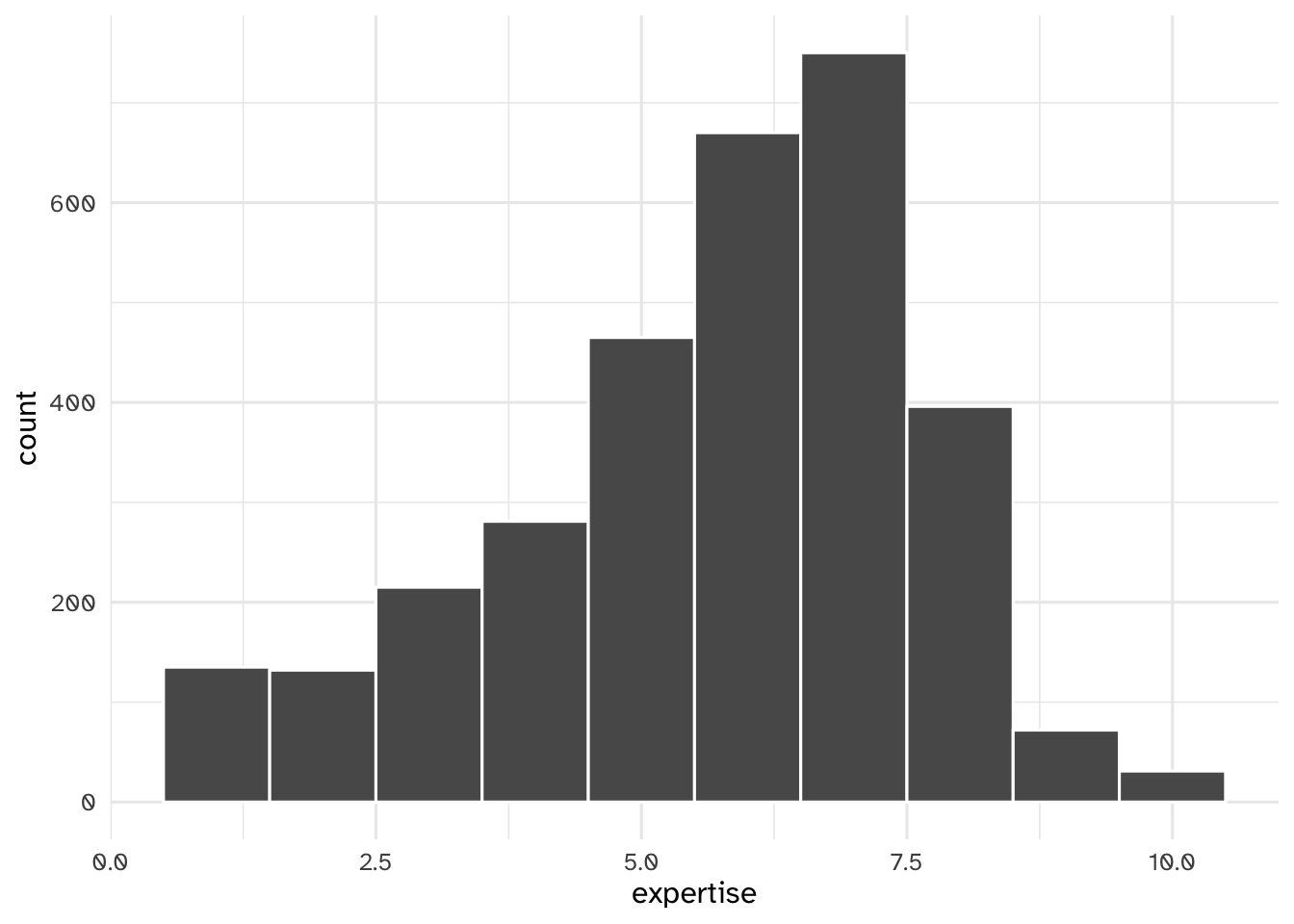
(ggplot(coffee_train) +
 geom_histogram(aes(x='expertise'), bins=10, color='white')).show()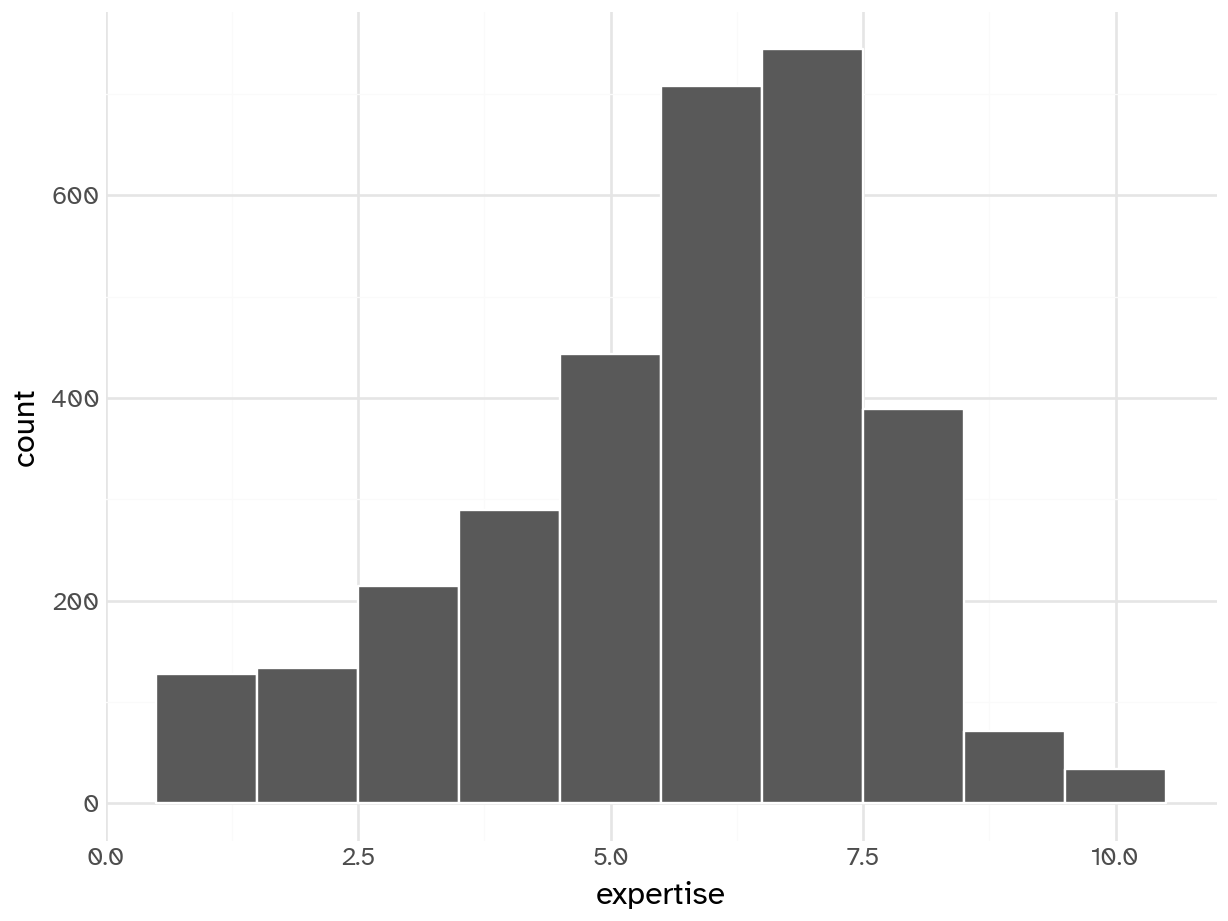
Add response here.
- Unimodal
- Slight skew (average expertise around 6)
- Few consider themselves experts
- Unsurprising, given the non-representative sample (who else would participate in a taste test except coffee enthusiasts?)
Your turn: Each coffee has three numeric ratings by the respondents: bitterness, acidity, and personal preference. Create a histogram for each of these characteristics, faceted by coffee type. What do you notice?
TipWrangling the data for easier visualization
The original structure of the data is one column for each coffee for each characteristic. You could create separate graphs for each of the 12 columns, but that seems like a lot of work. Instead, consider using the pivot_longer() function to restructure the data to one row per coffee per characteristic. This will make it easier to create the faceted histograms.
coffee_train |>
  select(starts_with("coffee"), -ends_with("notes")) |>
  pivot_longer(
    cols = everything(),
    names_to = c("coffee", "measure"),
    names_prefix = "coffee_",
    names_sep = "_",
    values_to = "value"
  )
# A tibble: 38,796 × 3
coffee measure value
<chr> <chr> <dbl>
1 a bitterness 2
2 a acidity 5
3 a personal 1
4 b bitterness 4
5 b acidity 1
6 b personal 4
7 c bitterness 2
8 c acidity 2
9 c personal 5
10 d bitterness 3
# ℹ 38,786 more rows# Select columns starting with "coffee" but not ending with "notes"
coffee_cols = [col for col in coffee_train.columns
if col.startswith('coffee_') and not col.endswith('_notes')]
# Reshape the data using melt (pandas equivalent of pivot_longer)
coffee_long = coffee_train[coffee_cols].melt(
var_name='coffee_measure',
value_name='value'
)
# Split the column names to separate coffee type and measure
coffee_long[['coffee', 'measure']] = coffee_long['coffee_measure'].str.replace('coffee_', '').str.split('_', n=1, expand=True)
# Drop the original combined column and reorder
coffee_long = coffee_long[['coffee', 'measure', 'value']]
coffee_long coffee measure value
0 a bitterness 1.0
1 a bitterness 3.0
2 a bitterness 1.0
3 a bitterness 1.0
4 a bitterness 1.0
... ... ... ...
38791 d personal_preference 5.0
38792 d personal_preference 1.0
38793 d personal_preference 2.0
38794 d personal_preference 5.0
38795 d personal_preference 4.0
[38796 rows x 3 columns]coffee_train |>
select(starts_with("coffee"), -ends_with("notes")) |>
pivot_longer(
cols = everything(),
names_to = c("coffee", "measure"),
names_prefix = "coffee_",
names_sep = "_",
values_to = "value"
) |>
ggplot(mapping = aes(x = value)) +
geom_bar() +
facet_grid(rows = vars(coffee), cols = vars(measure))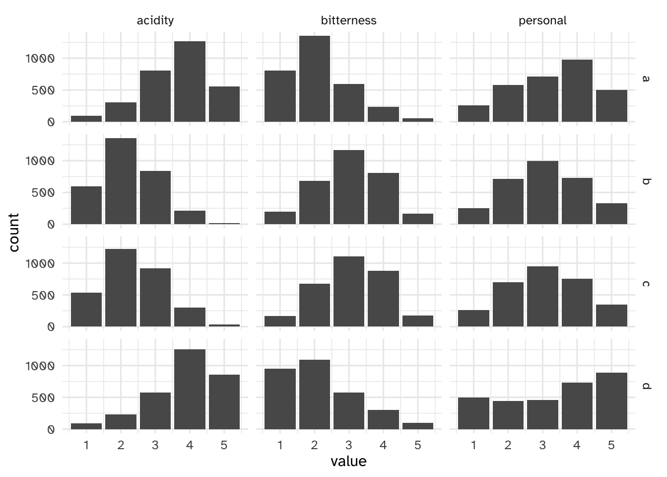
(ggplot(coffee_long) +
   geom_bar(aes(x='value')) +
   facet_grid('coffee ~ measure')).show()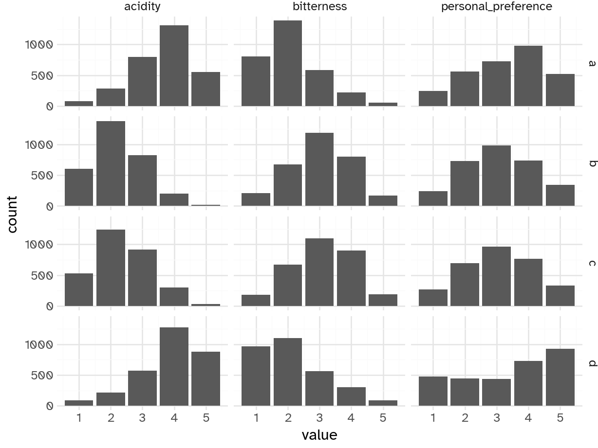
Add response here.
- Coffees A and D skew more acidic compared to B and C
- Coffees A and D are less bitter than B and C
- D tends to have higher personal preference, skews higher distribution overall
- A also skews a bit higher personal preference, whereas B and C are more normally distributed
Examining categorical variables
Your turn: Examine prefer_overall graphically. Record your observations.
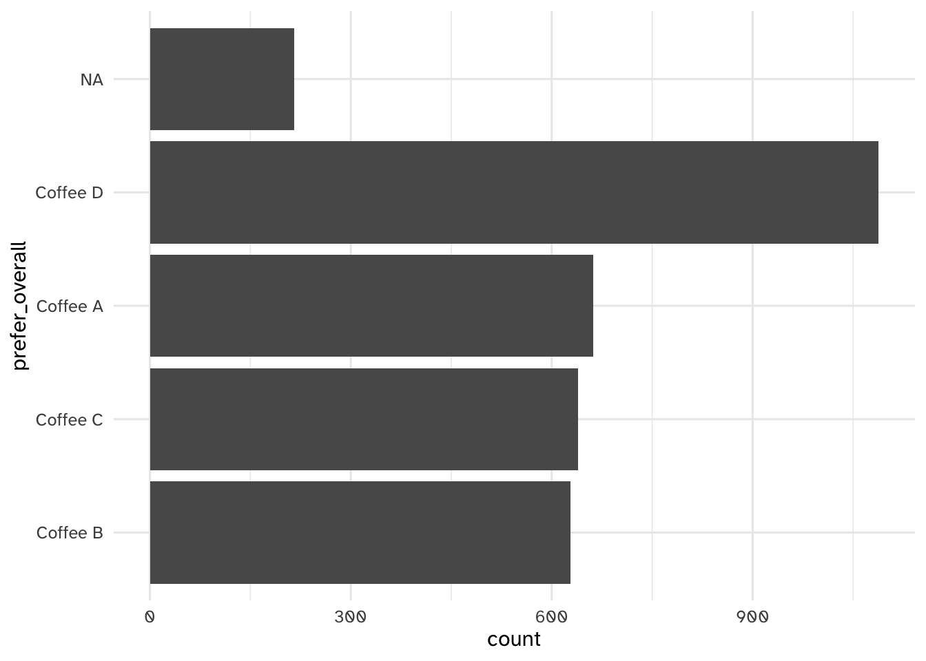
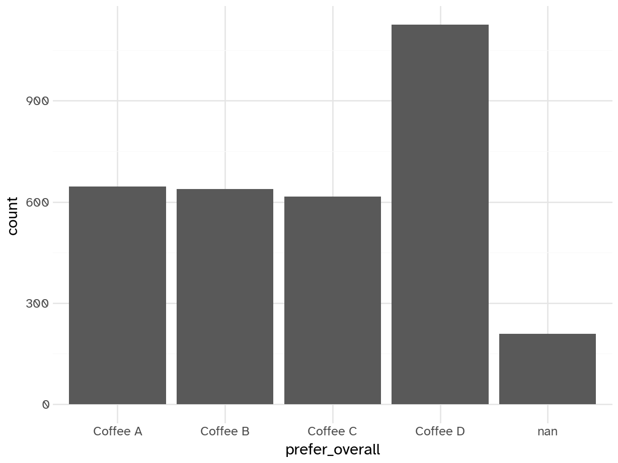
Add response here.
- Four possible choices - different kind of classification problem than in the past
- Coffee D is the most popular overall, similar levels of support for A/B/C
- Some respondents did not select any of the four - will need to drop in the modeling stage
- Is this preference gap large enough to necessitate undersampling or another class imbalance procedure?
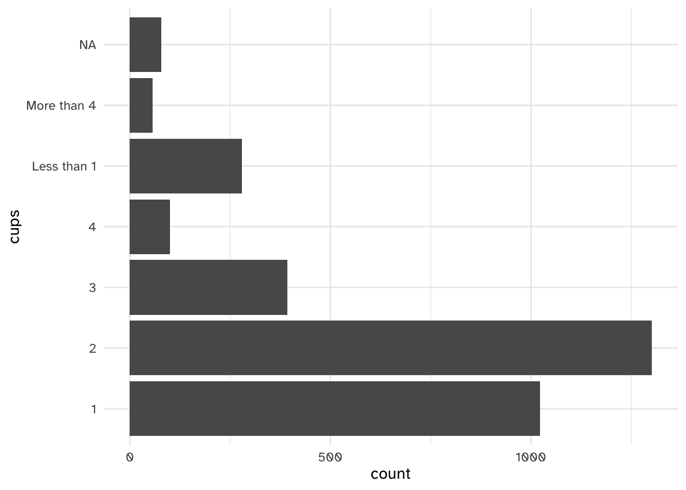
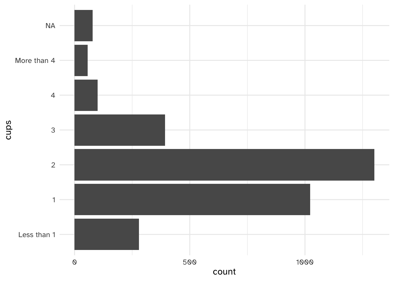
Your turn: Examine cups, brew, and roast_level. Record your observations, in particular how you might need to handle these variables in the modeling stage.
# cups
(ggplot(coffee_train) +
   geom_bar(aes(x='cups'))).show()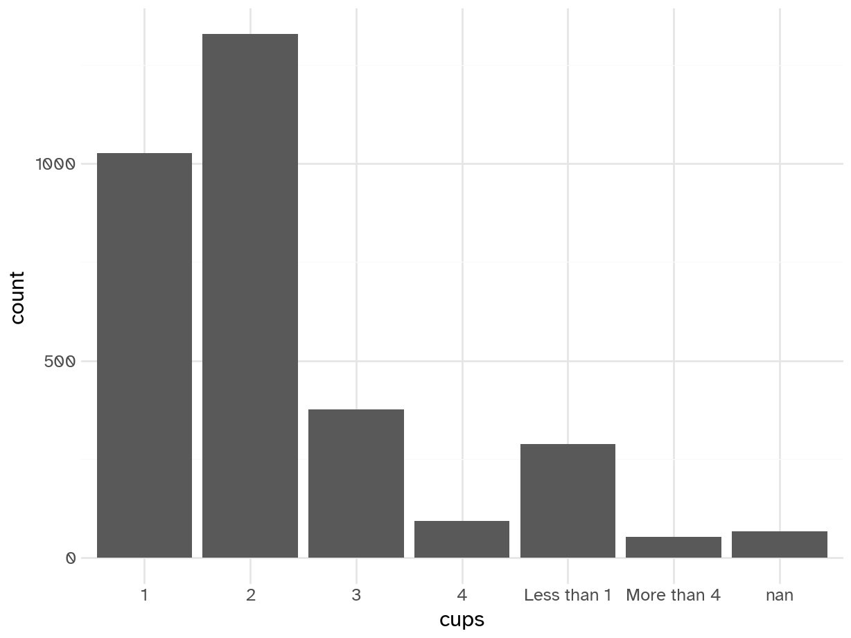
# correct order
coffee_train['cups'] = pd.Categorical(
    coffee_train['cups'],
    categories=["Less than 1", "1", "2", "3", "4", "More than 4"],
    ordered=True
)

(ggplot(coffee_train) +
   geom_bar(aes(x='cups'))).show()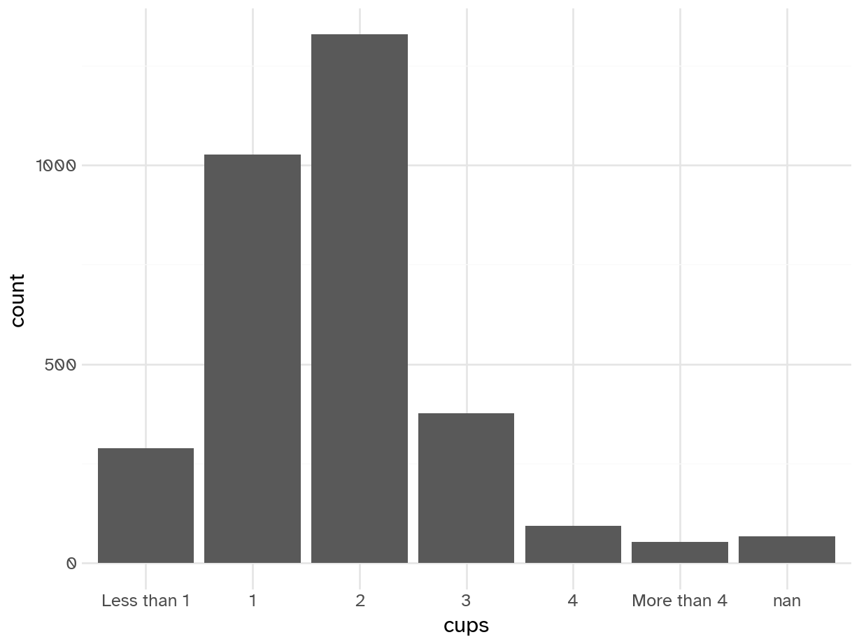
Add response here.
- Typical drinker is 1-2 cups per day
- A decent number of occasional coffee drinkers
- Long tail - some respondents drink a lot of coffee each day (I can’t imagine the number of bathroom trips…)
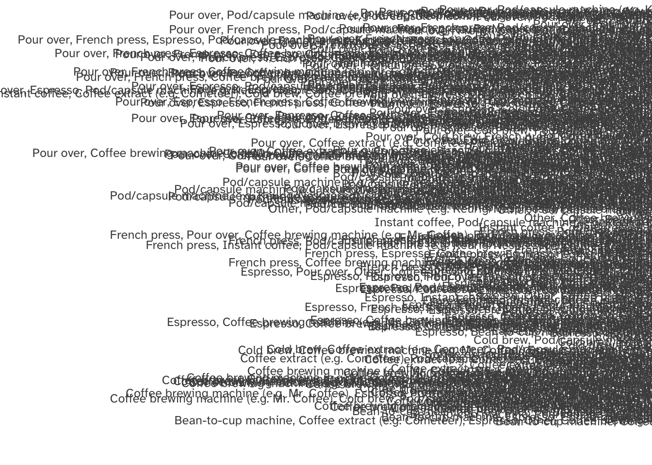
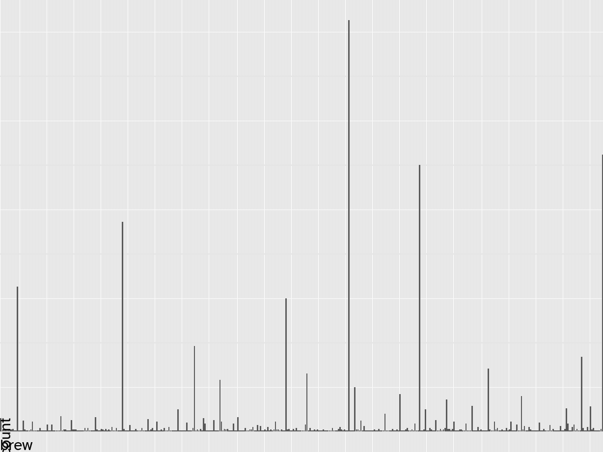
Add response here.
Oh crap. Each value contains potentially multiple types of brews. This is not useful in its current form. Need to split it up into one row per respondent per brew type.
coffee_train |>
  separate_longer_delim(
    cols = brew,
    delim = ", "
  ) |>
  mutate(brew = fct_infreq(brew) |> fct_rev()) |>
  ggplot(mapping = aes(y = brew)) +
  geom_bar()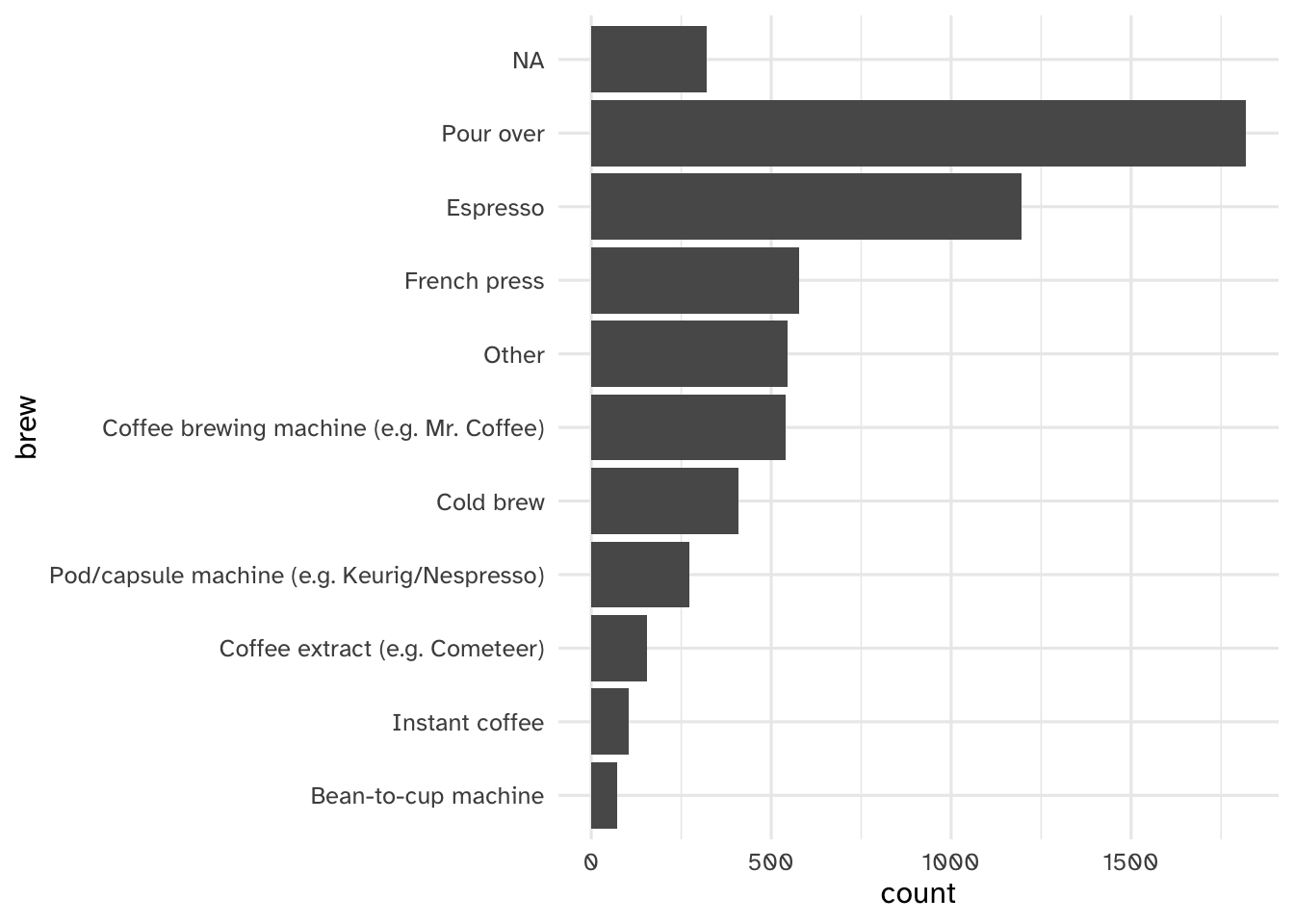
# Split brew column on delimiter and expand to multiple rows
coffee_brew_expanded = coffee_train.assign(
    brew=coffee_train['brew'].str.split(', ')
).explode('brew')

# Reorder by frequency (reversed for ascending frequency order)
brew_counts = coffee_brew_expanded['brew'].value_counts()
coffee_brew_expanded['brew'] = pd.Categorical(
    coffee_brew_expanded['brew'],
    categories=brew_counts.index.tolist()[::-1],
    ordered=True
)

# Create the plot
(ggplot(coffee_brew_expanded) +
  geom_bar(aes(x='brew'))).show()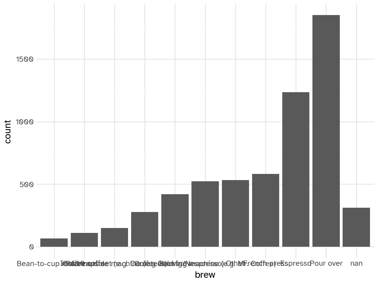
NoteBonus fun! How do the brew types correlate with one another?
This could be an issue later with modeling if we do dummy encoding.
library(ggcorrplot) # for the heatmap

coffee_train |>
  # get into a long format
  separate_longer_delim(
    cols = brew,
    delim = ", "
  ) |>
  # frequency count for each respondent and brew type
  count(submission_id, brew) |>
  # remove NAs
  drop_na() |>
  # restructure to one row per respondent, one column per brew type
  # fill in NAs with 0
  pivot_wider(names_from = brew, values_from = n, values_fill = 0) |>
  # drop submission_id - don't need anymore
  select(-submission_id) |>
  # calculate correlation coefficients
  cor() |>
  # draw the correlation matrix as a heatmap
  ggcorrplot(
    # order the variables by correlation values
    hc.order = TRUE,
    # just show the lower triangle
    type = "lower",
    # make each box a white border
    outline.color = "white"
  ) +
  # more optimal color palette
  scale_fill_continuous_diverging()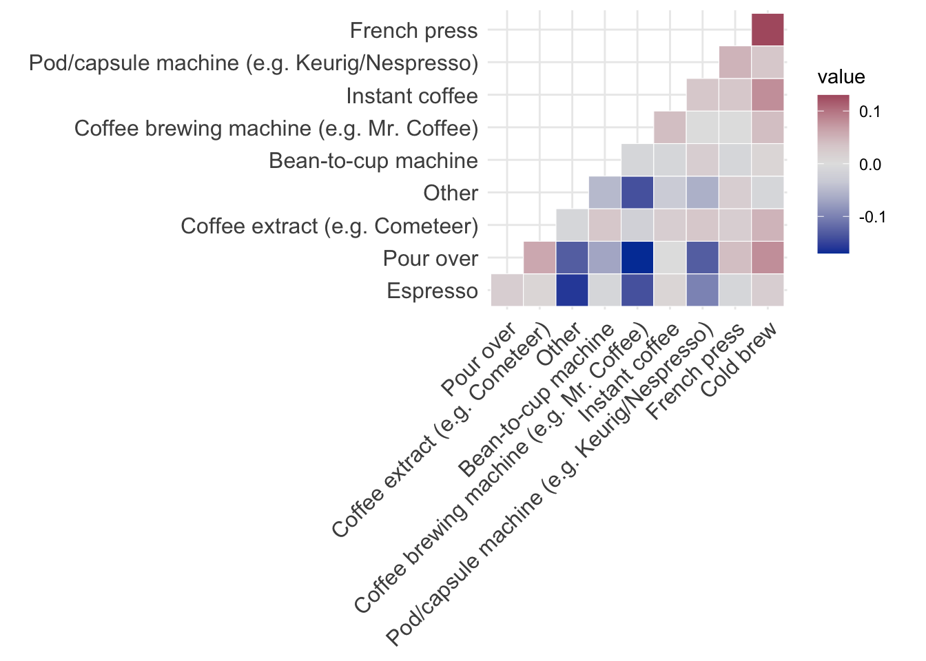
TODO
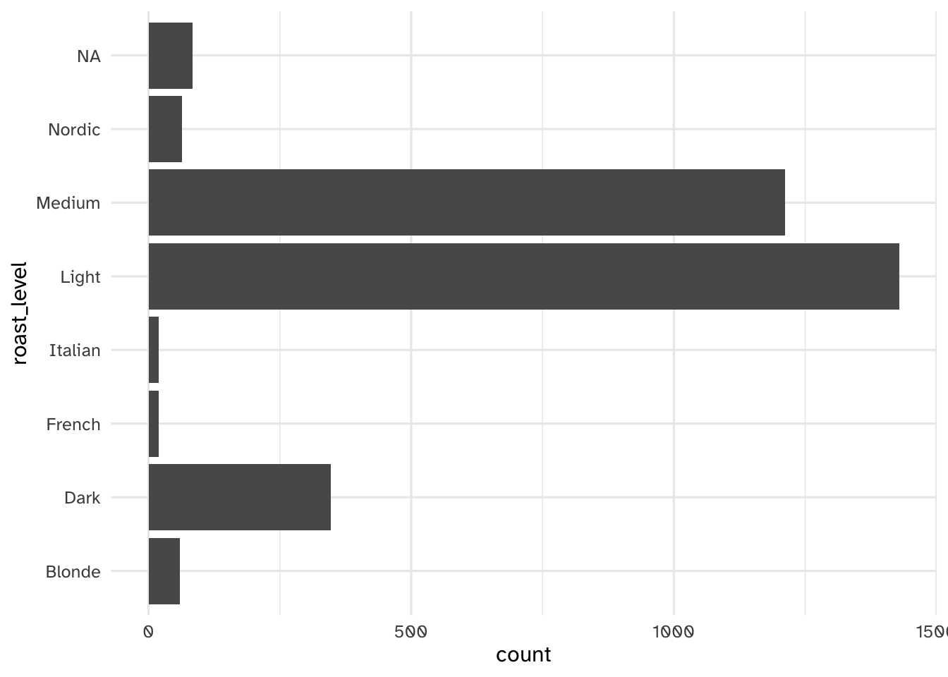
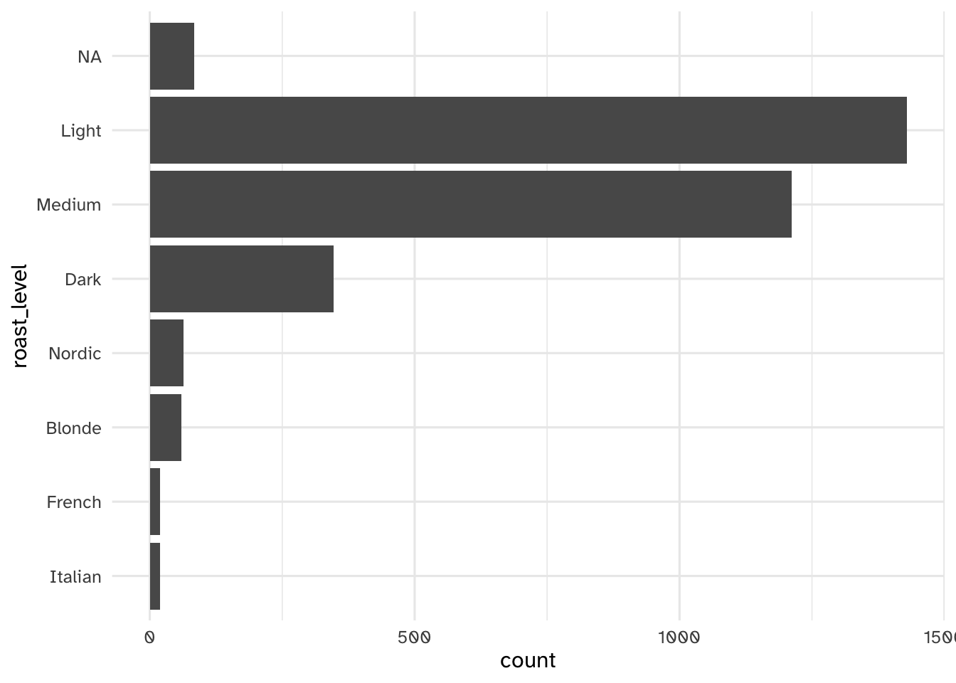
(ggplot(coffee_train) +
   geom_bar(aes(x='roast_level'))).show()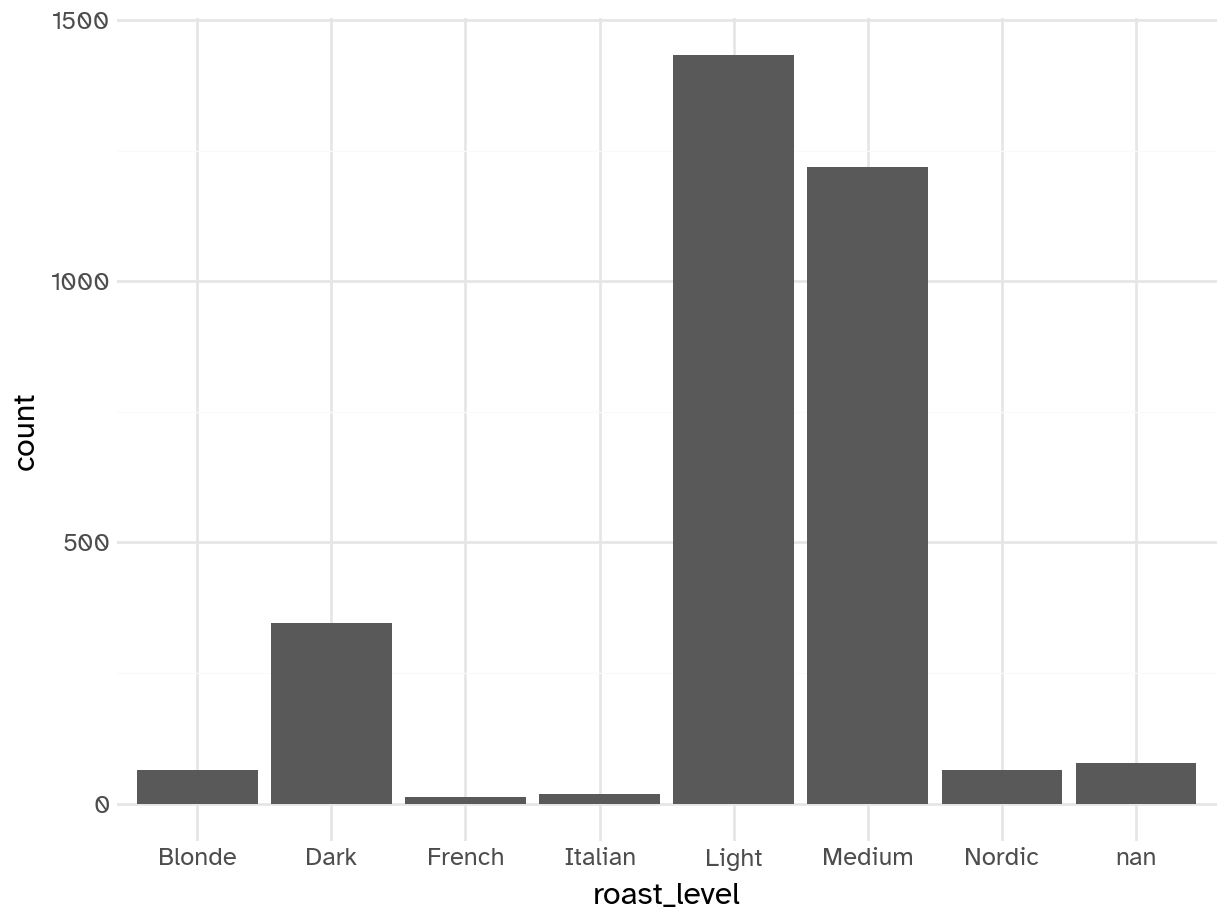
coffee_train['roast_level'] = pd.Categorical(
    coffee_train['roast_level'],
    categories=coffee_train['roast_level'].value_counts().index.tolist()[::-1],
    ordered=True)

(ggplot(coffee_train) +
   geom_bar(aes(x='roast_level'))).show()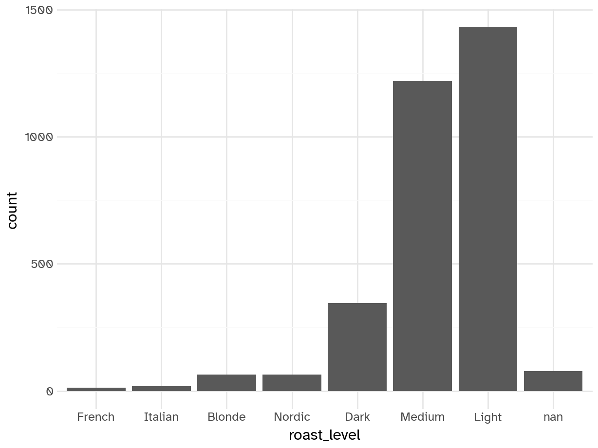
Add response here.
By far the most common roast preferences are light, medium, and dark. Others are so infrequent they might not be useful.
Some additional variables for fun
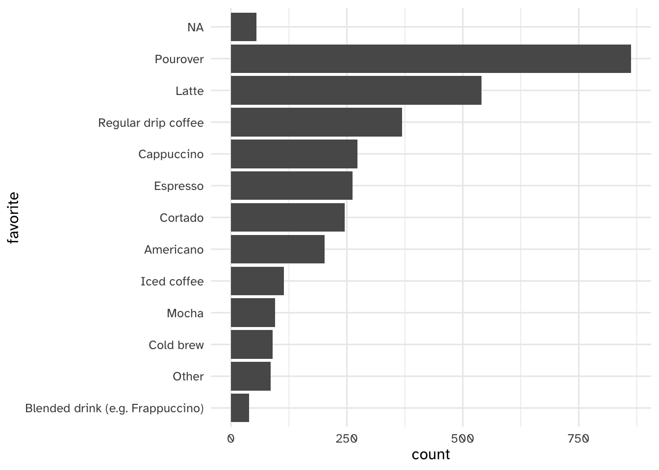
coffee_train['favorite'] = pd.Categorical(
    coffee_train['favorite'],
    categories=coffee_train['favorite'].value_counts().index.tolist()[::-1],
    ordered=True)

(ggplot(coffee_train) +
   geom_bar(aes(x='favorite'))).show()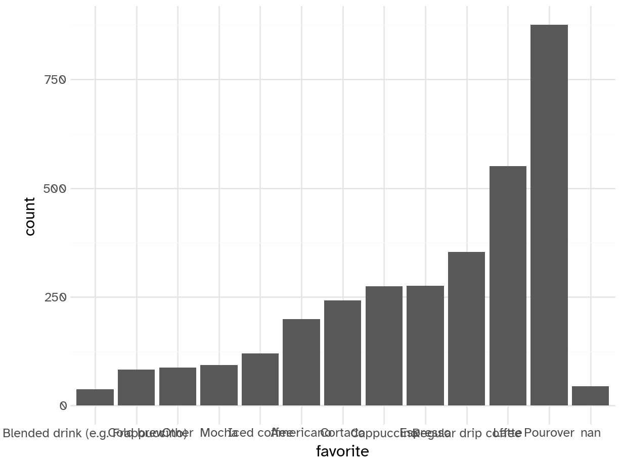
- Pourover is most popular (coffee snobs)
- Uneven distribution - some are distinctly less popular than others. Might be worth testing to collapse into “Other” category or hashing/effect encoding
- Not a ton of unique categories though
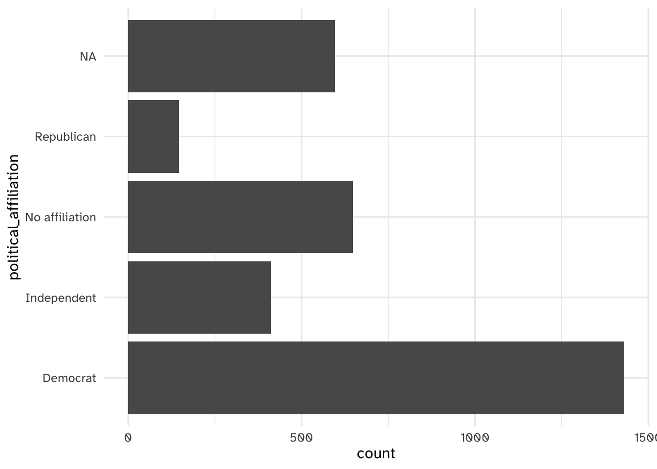
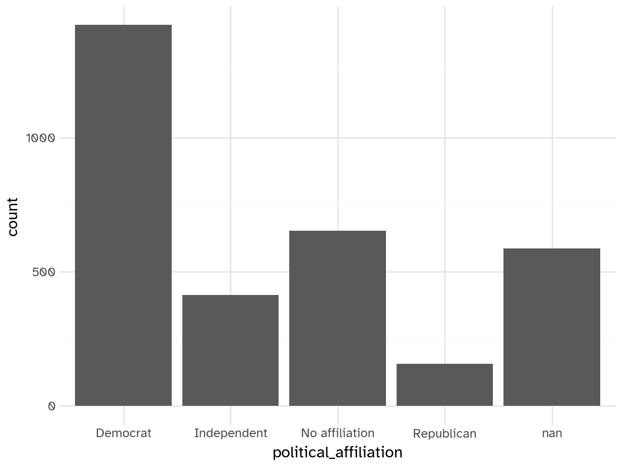
- Skews heavily Democratic
- Is this something that would even be useful?
Making comparisons
Your turn: Compare the relationship between coffee_d_personal_preference and the respondents’ preferred roast levels. Use a proportional bar chart to visualize the relationship.
Tip
Use position = "fill" with geom_bar() to automatically calculate percentages for the chart.
coffee_train |>
  filter(roast_level %in% c("Dark", "Medium", "Light")) |>
  mutate(
    roast_level = factor(roast_level, levels = c("Light", "Medium", "Dark"))
  ) |>
  ggplot(
    mapping = aes(y = coffee_d_personal_preference, fill = fct_rev(roast_level))
  ) +
  geom_bar(position = "fill") +
  scale_fill_discrete_sequential(rev = FALSE, guide = guide_legend(rev = TRUE))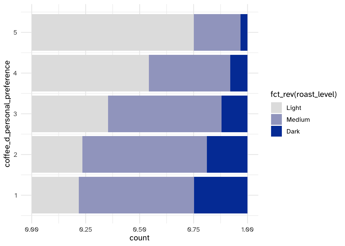
# Filter and prepare data
coffee_filtered = coffee_train[
    coffee_train['roast_level'].isin(['Dark', 'Medium', 'Light'])
].copy()

# Set roast_level as ordered categorical
coffee_filtered['roast_level'] = pd.Categorical(
    coffee_filtered['roast_level'],
    categories=['Light', 'Medium', 'Dark'],
    ordered=True
)

# Reverse roast_level for fill aesthetic
coffee_filtered['roast_level_rev'] = pd.Categorical(
    coffee_filtered['roast_level'],
    categories=['Dark', 'Medium', 'Light'],  # Reversed order
    ordered=True
)

# Create the proportional bar chart
(ggplot(coffee_filtered) +
  geom_bar(aes(x='coffee_d_personal_preference', fill='roast_level_rev'), position='fill')).show()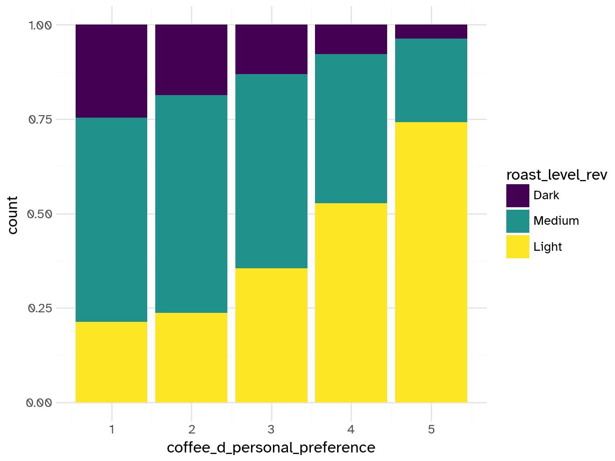
Add response here.
- People who prefer light roast tend to like coffee D more
- Those who like coffee D tend to prefer light or medium roasts
Your turn: Examine the relationship between the respondents’ numeric ratings for acidity, bitterness, and personal preference for each of the four coffees and compare to their overall preference. Record your observations.
pref_by_traits <- coffee_train |>
  select(starts_with("coffee"), -ends_with("notes"), prefer_overall) |>
  pivot_longer(
    cols = -prefer_overall,
    names_to = c("coffee", "measure"),
    names_prefix = "coffee_",
    names_sep = "_",
    values_to = "value"
  ) |>
  drop_na() |>
  mutate(coffee = fct_rev(coffee))

ggplot(data = pref_by_traits, mapping = aes(x = factor(value), y = coffee)) +
  geom_count() +
  facet_grid(rows = vars(prefer_overall), cols = vars(measure))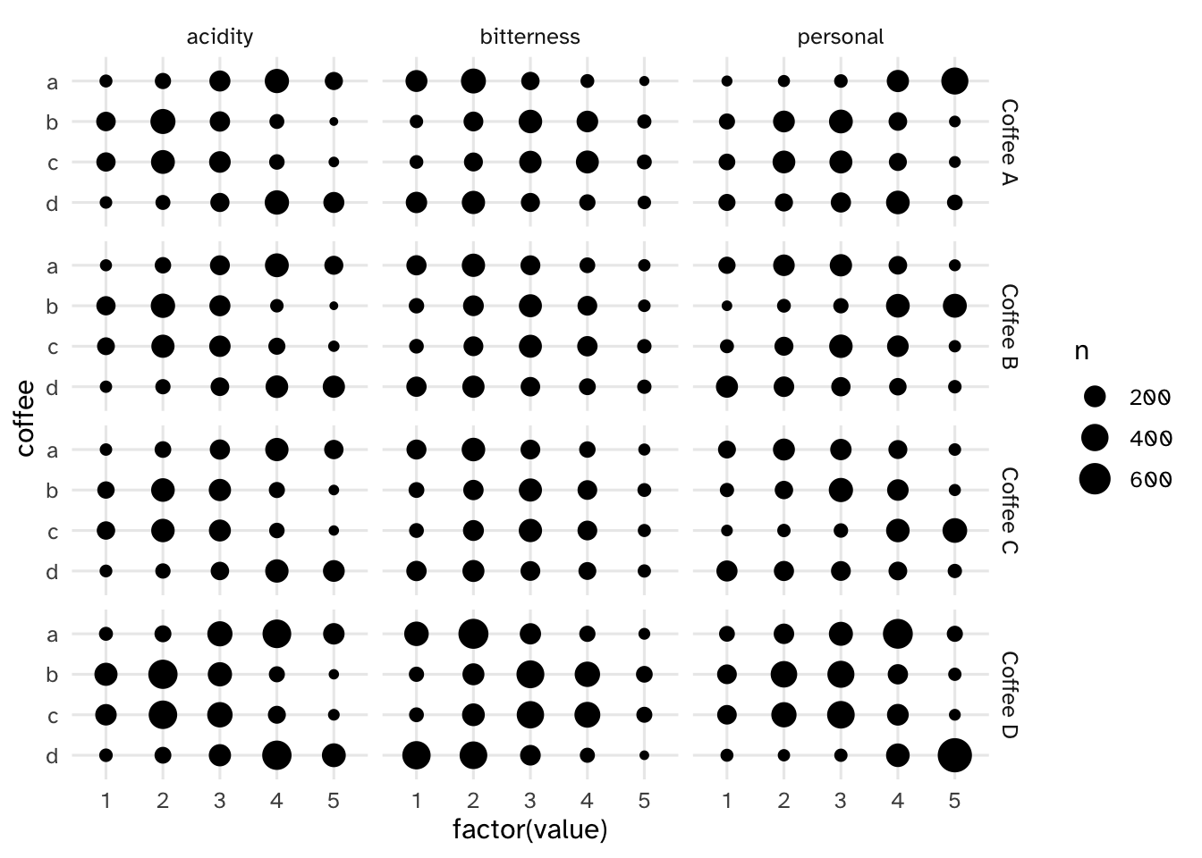
ggplot(data = pref_by_traits, mapping = aes(x = factor(value), y = coffee)) +
  geom_bin2d() +
  scale_fill_continuous_sequential() +
  facet_grid(rows = vars(prefer_overall), cols = vars(measure))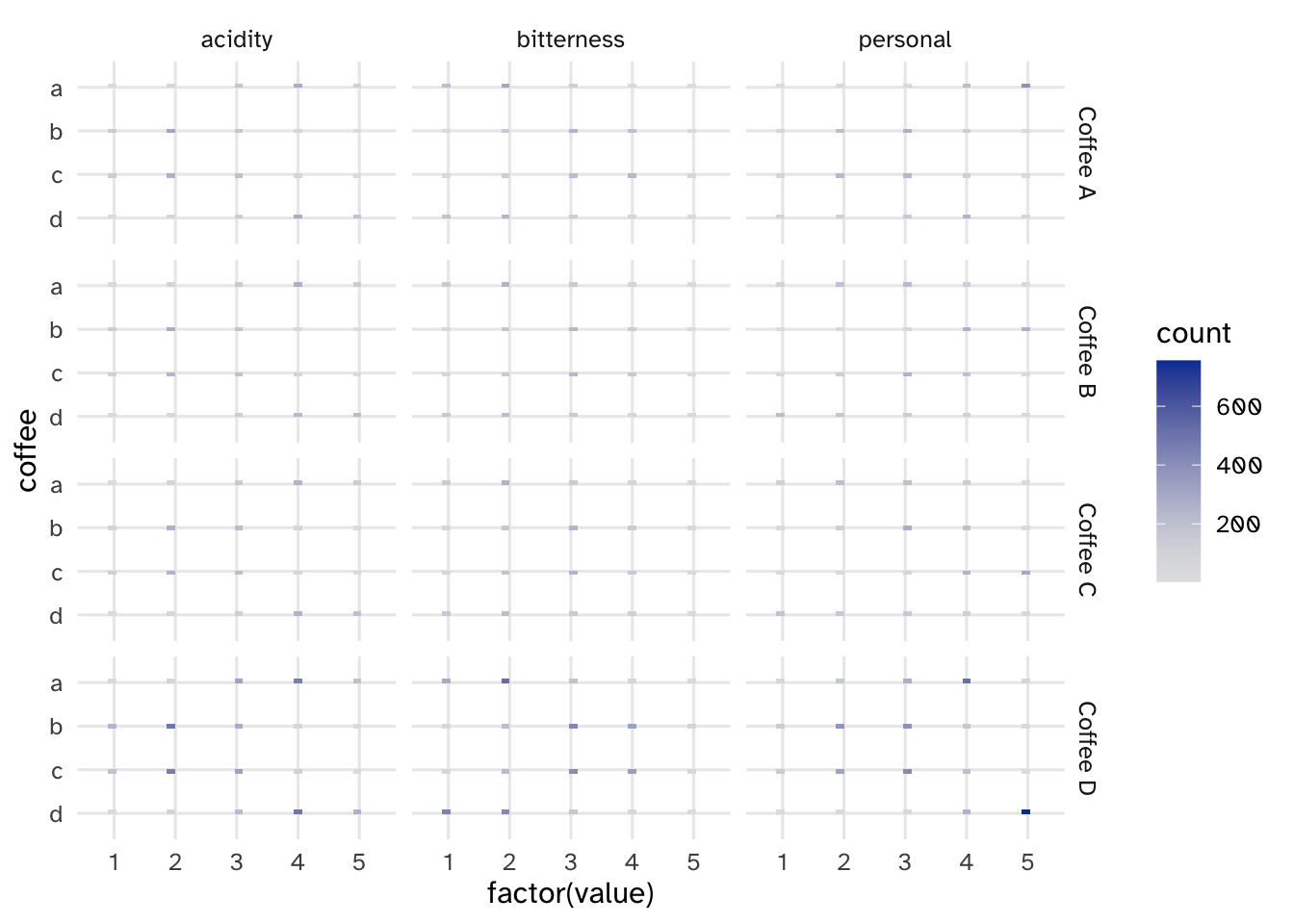
ggplot(
  data = pref_by_traits,
  mapping = aes(x = value, color = fct_rev(coffee))
) +
  geom_freqpoly(binwidth = 1) +
  scale_fill_discrete_qualitative() +
  facet_grid(rows = vars(prefer_overall), cols = vars(measure))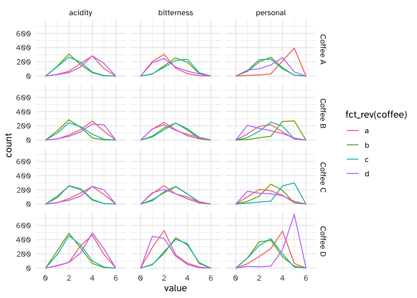
ggplot(data = pref_by_traits, mapping = aes(x = value, y = coffee)) +
  geom_boxplot() +
  facet_grid(rows = vars(prefer_overall), cols = vars(measure))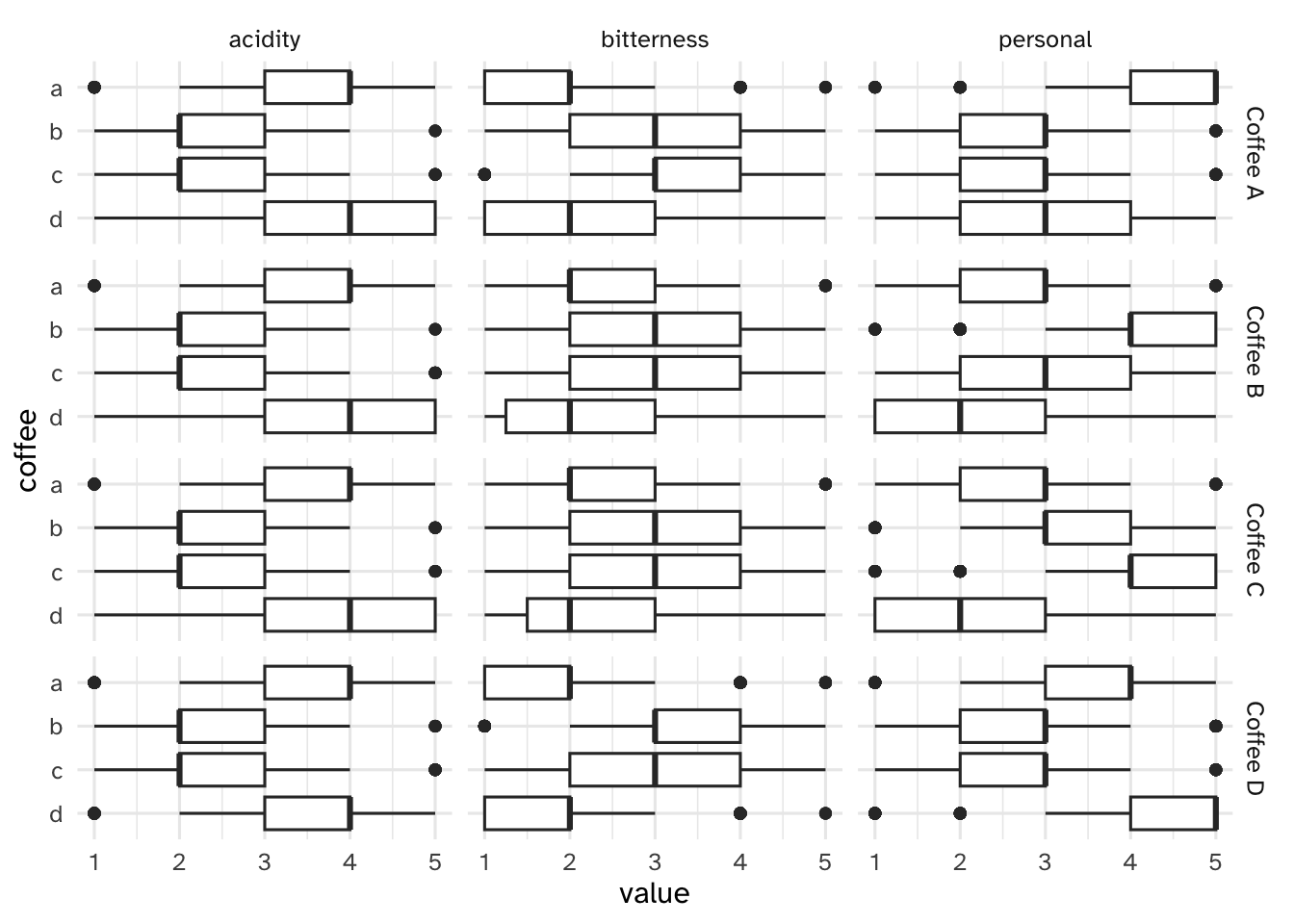
# Data preparation
coffee_cols = [col for col in coffee_train.columns
               if col.startswith('coffee_') and not col.endswith('_notes')]

pref_by_traits = coffee_train[coffee_cols + ['prefer_overall']].melt(
    id_vars=['prefer_overall'],
    var_name='coffee_measure',
    value_name='value'
).dropna()

# Split the column names to separate coffee type and measure
pref_by_traits[['coffee', 'measure']] = pref_by_traits['coffee_measure'].str.replace('coffee_', '').str.split('_', n=1, expand=True)

# Reverse coffee order for consistent ordering
coffee_order = ['d', 'c', 'b', 'a']
pref_by_traits['coffee'] = pd.Categorical(
    pref_by_traits['coffee'],
    categories=coffee_order,
    ordered=True
)

# Create the visualizations
# Plot 1: geom_count equivalent
(ggplot(pref_by_traits, aes(x='factor(value)', y='coffee')) +
  geom_count() +
  facet_grid('prefer_overall ~ measure')).show()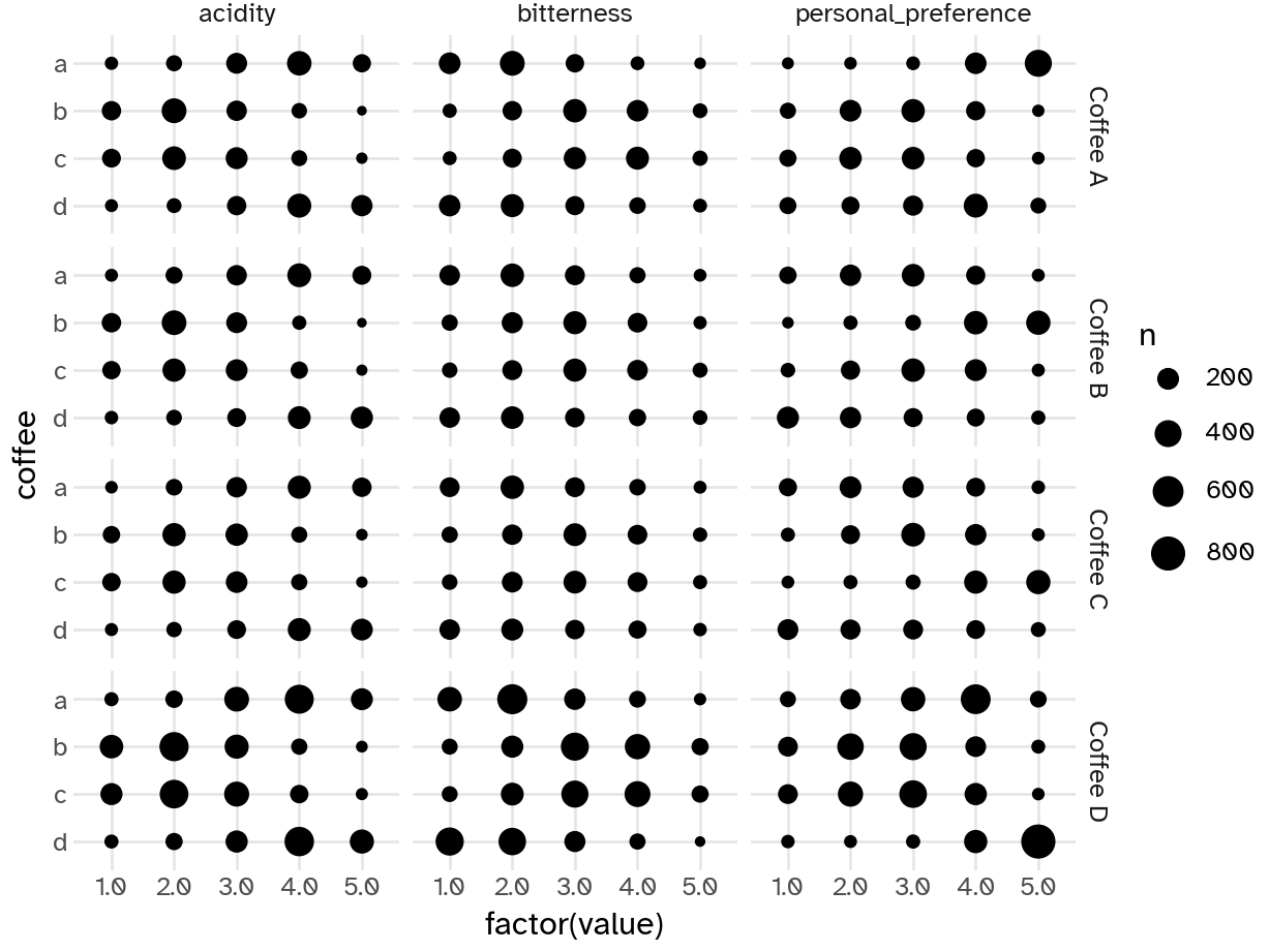
# Plot 2: geom_bin2d
(ggplot(pref_by_traits, aes(x='factor(value)', y='coffee')) +
  geom_bin2d() +
  facet_grid('prefer_overall ~ measure')).show()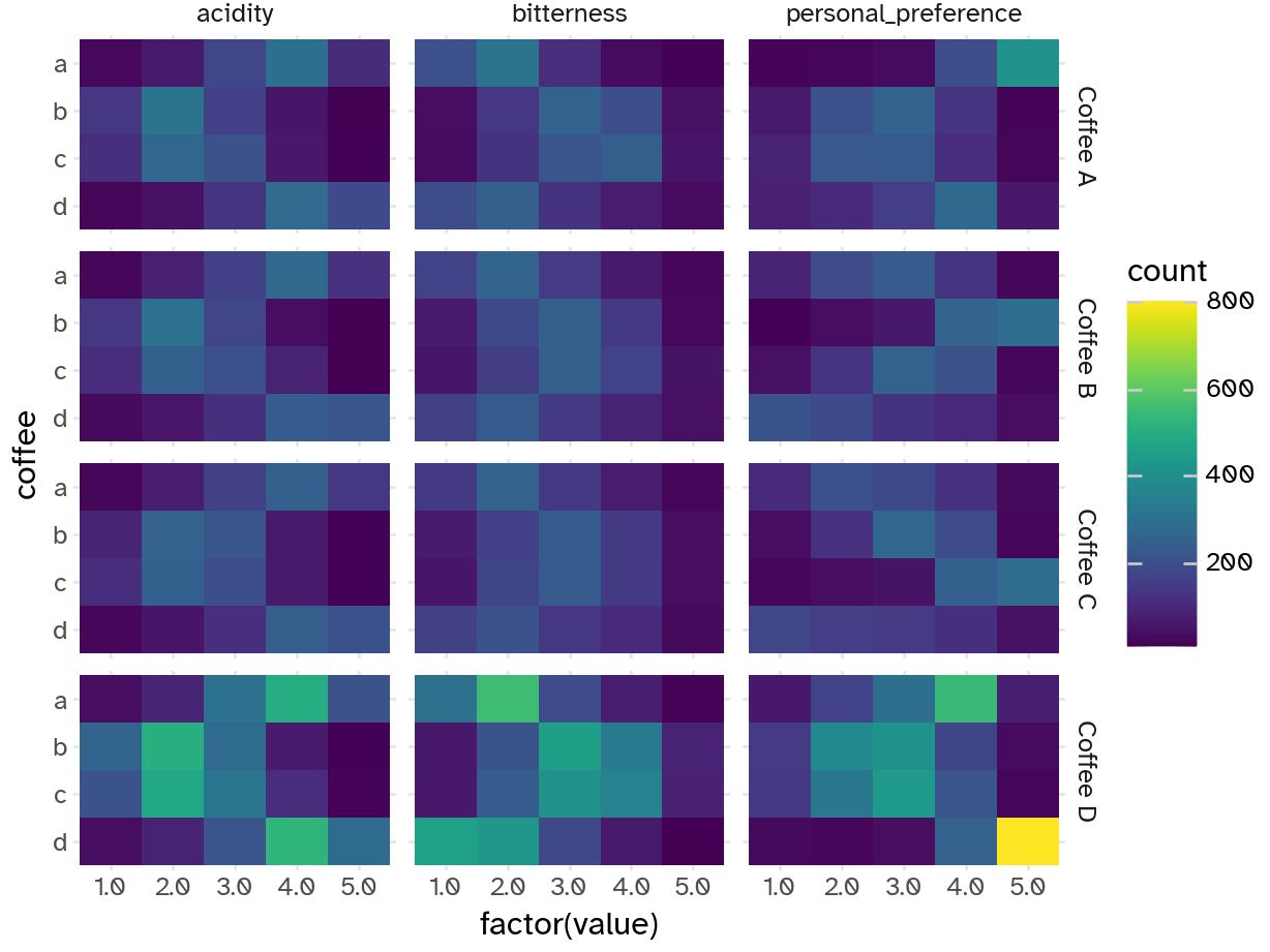
# Plot 3: geom_freqpoly
# Reverse coffee order for color mapping
pref_by_traits['coffee_rev'] = pd.Categorical(
    pref_by_traits['coffee'],
    categories=['d', 'c', 'b', 'a'],
    ordered=True
)

(ggplot(pref_by_traits, aes(x='value', color='coffee_rev')) +
  geom_freqpoly(binwidth=1) +
  facet_grid('prefer_overall ~ measure')).show()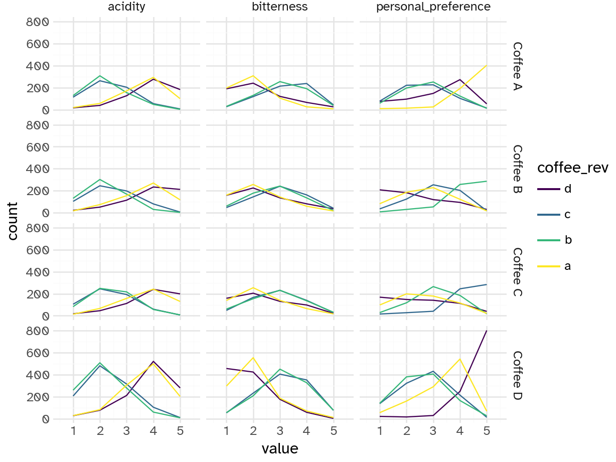
# Plot 4: geom_boxplot
(ggplot(pref_by_traits, aes(x='coffee', y='value')) +
  geom_boxplot() +
  facet_grid('prefer_overall ~ measure')).show()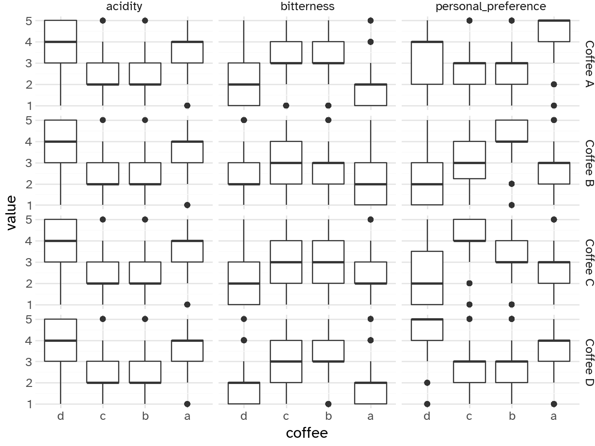
Add response here.
People who prefer coffee A
- Rate it higher for personal preference and acidity
- Rate it lower for bitterness
People who prefer coffee B
- Rate it higher for personal preference, mid for bitterness, and lower for acidity
People who prefer coffee C
- Rate it higher for personal preference, mid for bitterness, and lower for acidity
People who prefer coffee D
- Rate it higher for personal preference and acidity, lower for bitterness
Overall, seems like coffees A/D and B/C have similar evaluations
Data quality
Missingness
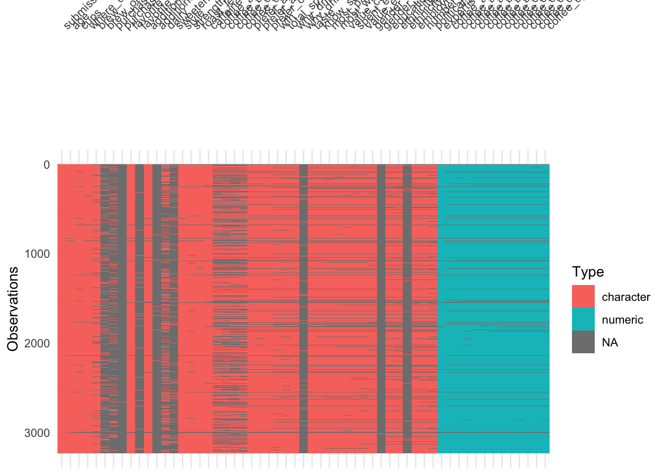
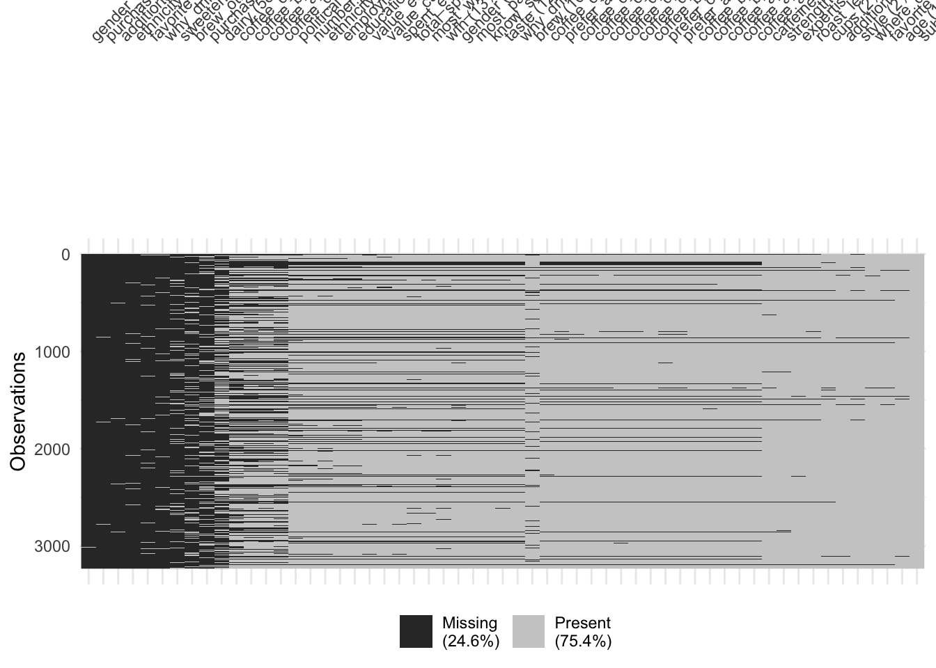
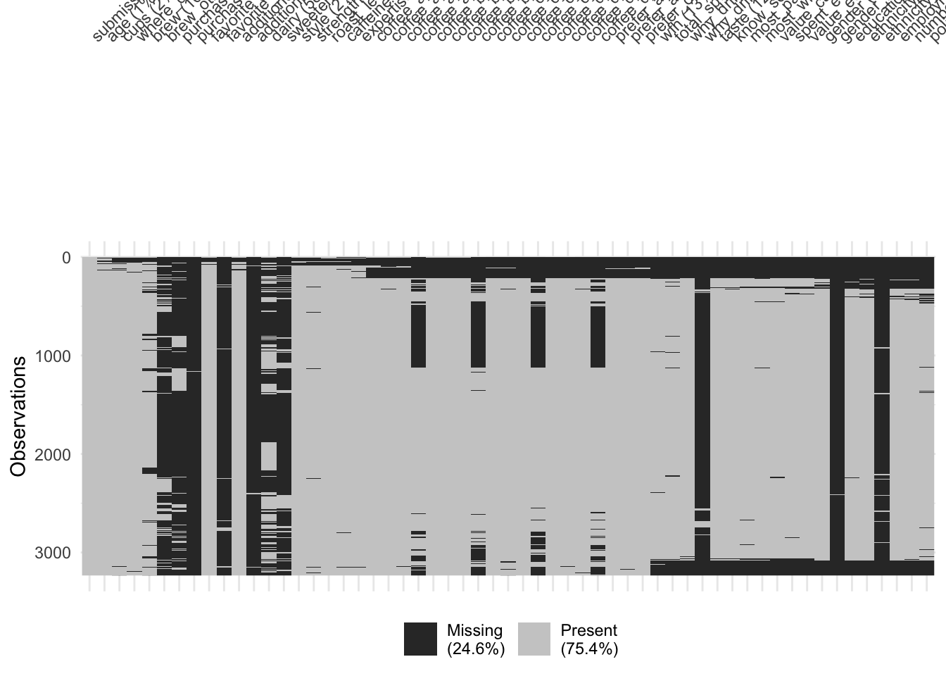
Demonstration: Use {visdat} or missingno to visualize missingness patterns in the data set.
import missingno as msno

# Quick glance of missingness by row/column order
msno.matrix(coffee_train)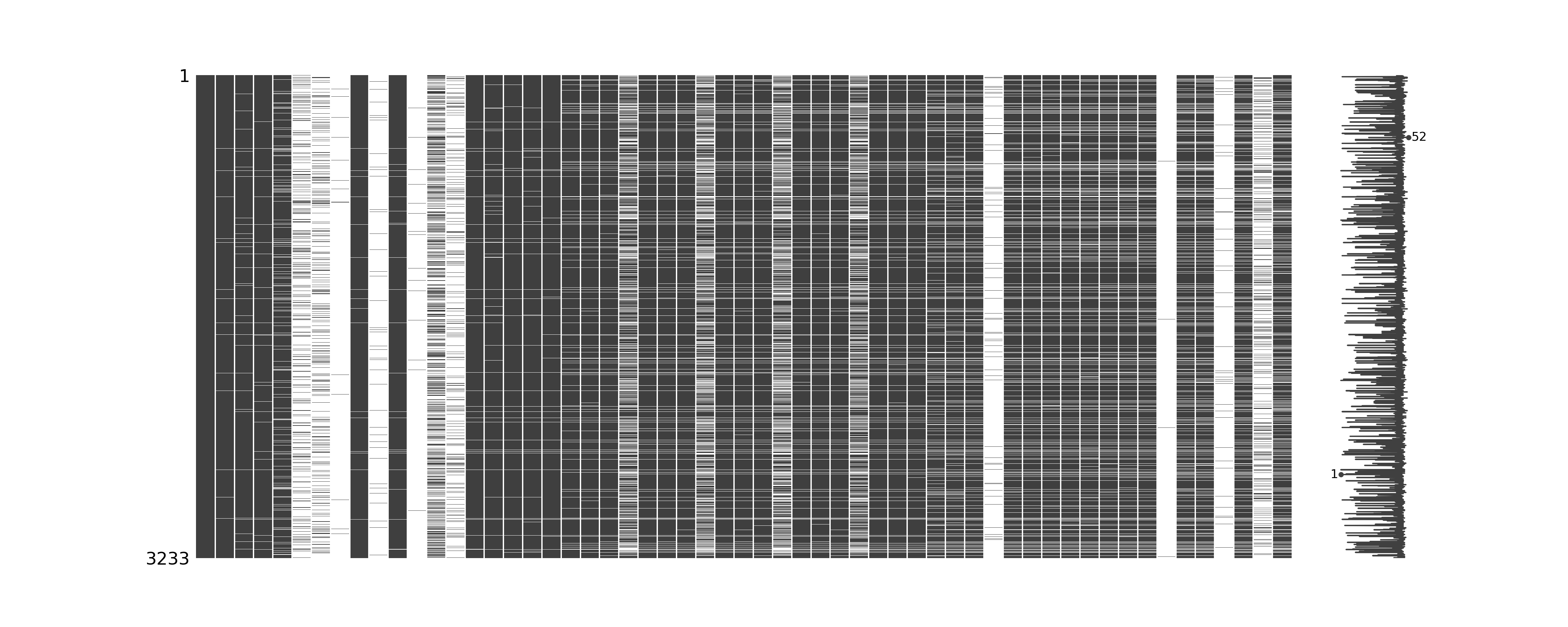
# Reorder columns based on % missing
msno.matrix(coffee_train.loc[:, coffee_train.isnull().sum().sort_values(ascending=False).index])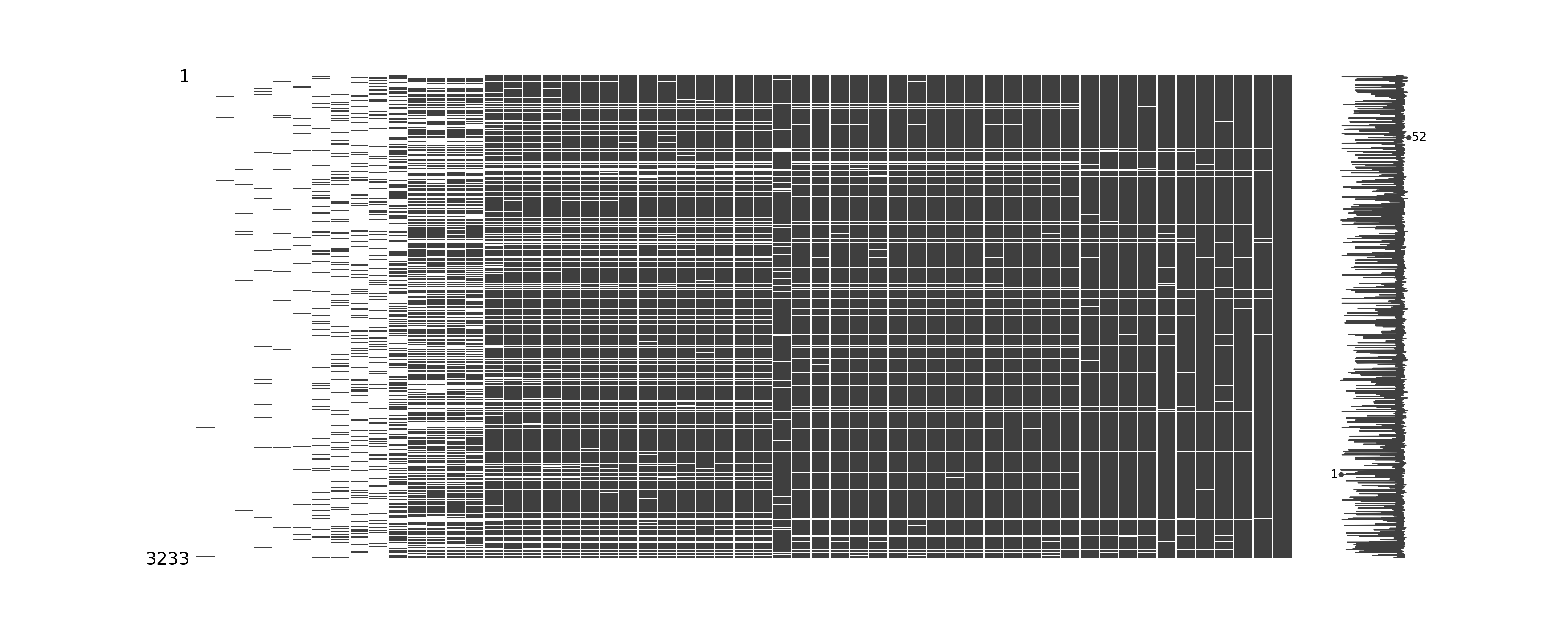
# Cluster rows based on similarity in missingness patterns
msno.dendrogram(coffee_train)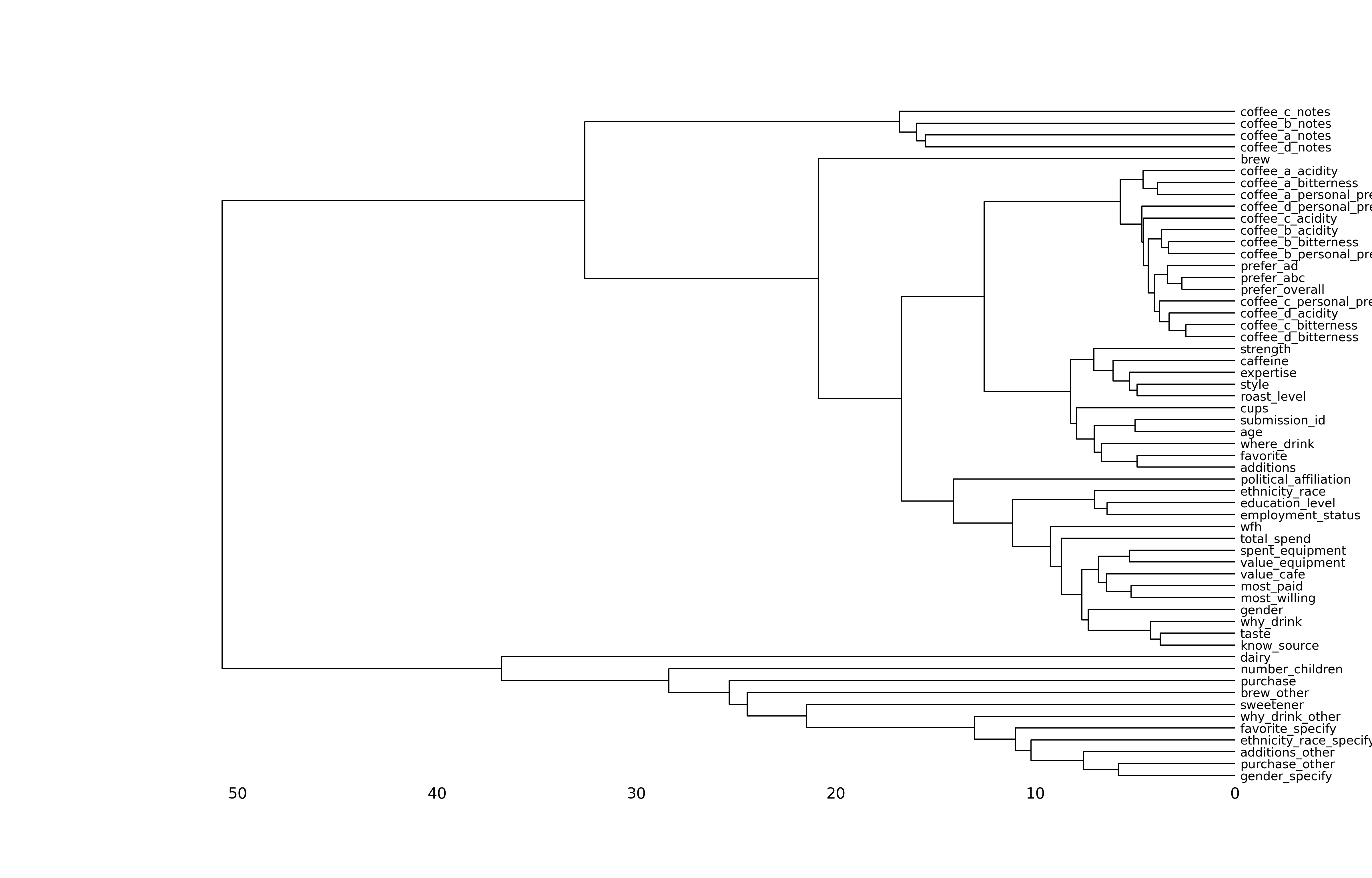
Your turn: Record your observations on the missingness patterns in the data set. What variables have high missingness? Is this surprising? What might you do to variables or observations with high degrees of missingness?
Add response here.
- Some missingness throughout the dataset
- Some variables are almost entirely missing (gender specify, lots of “other” columns). A lot of this is unsurprising since they are columns only to catch specific conditions or exceptions to other columns
- “Sweetener” is unusually high missingness - is this because people don’t use sweeteners or because they didn’t answer the question?
- Some observations have missing values for almost all the columns - are these valid observations? Is there enough info there to include in resulting models?
Outliers
Demonstration: Generate a scatterplot matrix for all the numeric variables in the data set.2
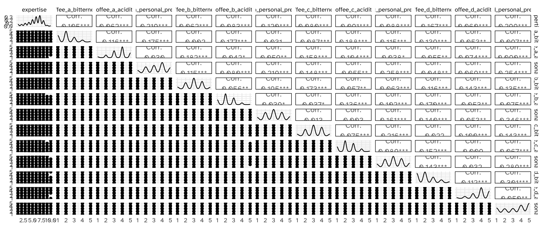
import matplotlib.pyplot as plt
from pandas.plotting import scatter_matrix

# Get all numeric columns
numeric_cols = coffee_train.select_dtypes(include=[np.number]).columns

# Create scatterplot matrix using pandas
fig, axes = plt.subplots(figsize=(15, 15))
scatter_matrix(coffee_train[numeric_cols], alpha=0.6, figsize=(15, 15), diagonal='hist')
array([[<Axes: xlabel='expertise', ylabel='expertise'>,
<Axes: xlabel='coffee_a_bitterness', ylabel='expertise'>,
<Axes: xlabel='coffee_a_acidity', ylabel='expertise'>,
<Axes: xlabel='coffee_a_personal_preference', ylabel='expertise'>,
<Axes: xlabel='coffee_b_bitterness', ylabel='expertise'>,
<Axes: xlabel='coffee_b_acidity', ylabel='expertise'>,
<Axes: xlabel='coffee_b_personal_preference', ylabel='expertise'>,
<Axes: xlabel='coffee_c_bitterness', ylabel='expertise'>,
<Axes: xlabel='coffee_c_acidity', ylabel='expertise'>,
<Axes: xlabel='coffee_c_personal_preference', ylabel='expertise'>,
<Axes: xlabel='coffee_d_bitterness', ylabel='expertise'>,
<Axes: xlabel='coffee_d_acidity', ylabel='expertise'>,
<Axes: xlabel='coffee_d_personal_preference', ylabel='expertise'>],
[<Axes: xlabel='expertise', ylabel='coffee_a_bitterness'>,
<Axes: xlabel='coffee_a_bitterness', ylabel='coffee_a_bitterness'>,
<Axes: xlabel='coffee_a_acidity', ylabel='coffee_a_bitterness'>,
<Axes: xlabel='coffee_a_personal_preference', ylabel='coffee_a_bitterness'>,
<Axes: xlabel='coffee_b_bitterness', ylabel='coffee_a_bitterness'>,
<Axes: xlabel='coffee_b_acidity', ylabel='coffee_a_bitterness'>,
<Axes: xlabel='coffee_b_personal_preference', ylabel='coffee_a_bitterness'>,
<Axes: xlabel='coffee_c_bitterness', ylabel='coffee_a_bitterness'>,
<Axes: xlabel='coffee_c_acidity', ylabel='coffee_a_bitterness'>,
<Axes: xlabel='coffee_c_personal_preference', ylabel='coffee_a_bitterness'>,
<Axes: xlabel='coffee_d_bitterness', ylabel='coffee_a_bitterness'>,
<Axes: xlabel='coffee_d_acidity', ylabel='coffee_a_bitterness'>,
<Axes: xlabel='coffee_d_personal_preference', ylabel='coffee_a_bitterness'>],
[<Axes: xlabel='expertise', ylabel='coffee_a_acidity'>,
<Axes: xlabel='coffee_a_bitterness', ylabel='coffee_a_acidity'>,
<Axes: xlabel='coffee_a_acidity', ylabel='coffee_a_acidity'>,
<Axes: xlabel='coffee_a_personal_preference', ylabel='coffee_a_acidity'>,
<Axes: xlabel='coffee_b_bitterness', ylabel='coffee_a_acidity'>,
<Axes: xlabel='coffee_b_acidity', ylabel='coffee_a_acidity'>,
<Axes: xlabel='coffee_b_personal_preference', ylabel='coffee_a_acidity'>,
<Axes: xlabel='coffee_c_bitterness', ylabel='coffee_a_acidity'>,
<Axes: xlabel='coffee_c_acidity', ylabel='coffee_a_acidity'>,
<Axes: xlabel='coffee_c_personal_preference', ylabel='coffee_a_acidity'>,
<Axes: xlabel='coffee_d_bitterness', ylabel='coffee_a_acidity'>,
<Axes: xlabel='coffee_d_acidity', ylabel='coffee_a_acidity'>,
<Axes: xlabel='coffee_d_personal_preference', ylabel='coffee_a_acidity'>],
[<Axes: xlabel='expertise', ylabel='coffee_a_personal_preference'>,
<Axes: xlabel='coffee_a_bitterness', ylabel='coffee_a_personal_preference'>,
<Axes: xlabel='coffee_a_acidity', ylabel='coffee_a_personal_preference'>,
<Axes: xlabel='coffee_a_personal_preference', ylabel='coffee_a_personal_preference'>,
<Axes: xlabel='coffee_b_bitterness', ylabel='coffee_a_personal_preference'>,
<Axes: xlabel='coffee_b_acidity', ylabel='coffee_a_personal_preference'>,
<Axes: xlabel='coffee_b_personal_preference', ylabel='coffee_a_personal_preference'>,
<Axes: xlabel='coffee_c_bitterness', ylabel='coffee_a_personal_preference'>,
<Axes: xlabel='coffee_c_acidity', ylabel='coffee_a_personal_preference'>,
<Axes: xlabel='coffee_c_personal_preference', ylabel='coffee_a_personal_preference'>,
<Axes: xlabel='coffee_d_bitterness', ylabel='coffee_a_personal_preference'>,
<Axes: xlabel='coffee_d_acidity', ylabel='coffee_a_personal_preference'>,
<Axes: xlabel='coffee_d_personal_preference', ylabel='coffee_a_personal_preference'>],
[<Axes: xlabel='expertise', ylabel='coffee_b_bitterness'>,
<Axes: xlabel='coffee_a_bitterness', ylabel='coffee_b_bitterness'>,
<Axes: xlabel='coffee_a_acidity', ylabel='coffee_b_bitterness'>,
<Axes: xlabel='coffee_a_personal_preference', ylabel='coffee_b_bitterness'>,
<Axes: xlabel='coffee_b_bitterness', ylabel='coffee_b_bitterness'>,
<Axes: xlabel='coffee_b_acidity', ylabel='coffee_b_bitterness'>,
<Axes: xlabel='coffee_b_personal_preference', ylabel='coffee_b_bitterness'>,
<Axes: xlabel='coffee_c_bitterness', ylabel='coffee_b_bitterness'>,
<Axes: xlabel='coffee_c_acidity', ylabel='coffee_b_bitterness'>,
<Axes: xlabel='coffee_c_personal_preference', ylabel='coffee_b_bitterness'>,
<Axes: xlabel='coffee_d_bitterness', ylabel='coffee_b_bitterness'>,
<Axes: xlabel='coffee_d_acidity', ylabel='coffee_b_bitterness'>,
<Axes: xlabel='coffee_d_personal_preference', ylabel='coffee_b_bitterness'>],
[<Axes: xlabel='expertise', ylabel='coffee_b_acidity'>,
<Axes: xlabel='coffee_a_bitterness', ylabel='coffee_b_acidity'>,
<Axes: xlabel='coffee_a_acidity', ylabel='coffee_b_acidity'>,
<Axes: xlabel='coffee_a_personal_preference', ylabel='coffee_b_acidity'>,
<Axes: xlabel='coffee_b_bitterness', ylabel='coffee_b_acidity'>,
<Axes: xlabel='coffee_b_acidity', ylabel='coffee_b_acidity'>,
<Axes: xlabel='coffee_b_personal_preference', ylabel='coffee_b_acidity'>,
<Axes: xlabel='coffee_c_bitterness', ylabel='coffee_b_acidity'>,
<Axes: xlabel='coffee_c_acidity', ylabel='coffee_b_acidity'>,
<Axes: xlabel='coffee_c_personal_preference', ylabel='coffee_b_acidity'>,
<Axes: xlabel='coffee_d_bitterness', ylabel='coffee_b_acidity'>,
<Axes: xlabel='coffee_d_acidity', ylabel='coffee_b_acidity'>,
<Axes: xlabel='coffee_d_personal_preference', ylabel='coffee_b_acidity'>],
[<Axes: xlabel='expertise', ylabel='coffee_b_personal_preference'>,
<Axes: xlabel='coffee_a_bitterness', ylabel='coffee_b_personal_preference'>,
<Axes: xlabel='coffee_a_acidity', ylabel='coffee_b_personal_preference'>,
<Axes: xlabel='coffee_a_personal_preference', ylabel='coffee_b_personal_preference'>,
<Axes: xlabel='coffee_b_bitterness', ylabel='coffee_b_personal_preference'>,
<Axes: xlabel='coffee_b_acidity', ylabel='coffee_b_personal_preference'>,
<Axes: xlabel='coffee_b_personal_preference', ylabel='coffee_b_personal_preference'>,
<Axes: xlabel='coffee_c_bitterness', ylabel='coffee_b_personal_preference'>,
<Axes: xlabel='coffee_c_acidity', ylabel='coffee_b_personal_preference'>,
<Axes: xlabel='coffee_c_personal_preference', ylabel='coffee_b_personal_preference'>,
<Axes: xlabel='coffee_d_bitterness', ylabel='coffee_b_personal_preference'>,
<Axes: xlabel='coffee_d_acidity', ylabel='coffee_b_personal_preference'>,
<Axes: xlabel='coffee_d_personal_preference', ylabel='coffee_b_personal_preference'>],
[<Axes: xlabel='expertise', ylabel='coffee_c_bitterness'>,
<Axes: xlabel='coffee_a_bitterness', ylabel='coffee_c_bitterness'>,
<Axes: xlabel='coffee_a_acidity', ylabel='coffee_c_bitterness'>,
<Axes: xlabel='coffee_a_personal_preference', ylabel='coffee_c_bitterness'>,
<Axes: xlabel='coffee_b_bitterness', ylabel='coffee_c_bitterness'>,
<Axes: xlabel='coffee_b_acidity', ylabel='coffee_c_bitterness'>,
<Axes: xlabel='coffee_b_personal_preference', ylabel='coffee_c_bitterness'>,
<Axes: xlabel='coffee_c_bitterness', ylabel='coffee_c_bitterness'>,
<Axes: xlabel='coffee_c_acidity', ylabel='coffee_c_bitterness'>,
<Axes: xlabel='coffee_c_personal_preference', ylabel='coffee_c_bitterness'>,
<Axes: xlabel='coffee_d_bitterness', ylabel='coffee_c_bitterness'>,
<Axes: xlabel='coffee_d_acidity', ylabel='coffee_c_bitterness'>,
<Axes: xlabel='coffee_d_personal_preference', ylabel='coffee_c_bitterness'>],
[<Axes: xlabel='expertise', ylabel='coffee_c_acidity'>,
<Axes: xlabel='coffee_a_bitterness', ylabel='coffee_c_acidity'>,
<Axes: xlabel='coffee_a_acidity', ylabel='coffee_c_acidity'>,
<Axes: xlabel='coffee_a_personal_preference', ylabel='coffee_c_acidity'>,
<Axes: xlabel='coffee_b_bitterness', ylabel='coffee_c_acidity'>,
<Axes: xlabel='coffee_b_acidity', ylabel='coffee_c_acidity'>,
<Axes: xlabel='coffee_b_personal_preference', ylabel='coffee_c_acidity'>,
<Axes: xlabel='coffee_c_bitterness', ylabel='coffee_c_acidity'>,
<Axes: xlabel='coffee_c_acidity', ylabel='coffee_c_acidity'>,
<Axes: xlabel='coffee_c_personal_preference', ylabel='coffee_c_acidity'>,
<Axes: xlabel='coffee_d_bitterness', ylabel='coffee_c_acidity'>,
<Axes: xlabel='coffee_d_acidity', ylabel='coffee_c_acidity'>,
<Axes: xlabel='coffee_d_personal_preference', ylabel='coffee_c_acidity'>],
[<Axes: xlabel='expertise', ylabel='coffee_c_personal_preference'>,
<Axes: xlabel='coffee_a_bitterness', ylabel='coffee_c_personal_preference'>,
<Axes: xlabel='coffee_a_acidity', ylabel='coffee_c_personal_preference'>,
<Axes: xlabel='coffee_a_personal_preference', ylabel='coffee_c_personal_preference'>,
<Axes: xlabel='coffee_b_bitterness', ylabel='coffee_c_personal_preference'>,
<Axes: xlabel='coffee_b_acidity', ylabel='coffee_c_personal_preference'>,
<Axes: xlabel='coffee_b_personal_preference', ylabel='coffee_c_personal_preference'>,
<Axes: xlabel='coffee_c_bitterness', ylabel='coffee_c_personal_preference'>,
<Axes: xlabel='coffee_c_acidity', ylabel='coffee_c_personal_preference'>,
<Axes: xlabel='coffee_c_personal_preference', ylabel='coffee_c_personal_preference'>,
<Axes: xlabel='coffee_d_bitterness', ylabel='coffee_c_personal_preference'>,
<Axes: xlabel='coffee_d_acidity', ylabel='coffee_c_personal_preference'>,
<Axes: xlabel='coffee_d_personal_preference', ylabel='coffee_c_personal_preference'>],
[<Axes: xlabel='expertise', ylabel='coffee_d_bitterness'>,
<Axes: xlabel='coffee_a_bitterness', ylabel='coffee_d_bitterness'>,
<Axes: xlabel='coffee_a_acidity', ylabel='coffee_d_bitterness'>,
<Axes: xlabel='coffee_a_personal_preference', ylabel='coffee_d_bitterness'>,
<Axes: xlabel='coffee_b_bitterness', ylabel='coffee_d_bitterness'>,
<Axes: xlabel='coffee_b_acidity', ylabel='coffee_d_bitterness'>,
<Axes: xlabel='coffee_b_personal_preference', ylabel='coffee_d_bitterness'>,
<Axes: xlabel='coffee_c_bitterness', ylabel='coffee_d_bitterness'>,
<Axes: xlabel='coffee_c_acidity', ylabel='coffee_d_bitterness'>,
<Axes: xlabel='coffee_c_personal_preference', ylabel='coffee_d_bitterness'>,
<Axes: xlabel='coffee_d_bitterness', ylabel='coffee_d_bitterness'>,
<Axes: xlabel='coffee_d_acidity', ylabel='coffee_d_bitterness'>,
<Axes: xlabel='coffee_d_personal_preference', ylabel='coffee_d_bitterness'>],
[<Axes: xlabel='expertise', ylabel='coffee_d_acidity'>,
<Axes: xlabel='coffee_a_bitterness', ylabel='coffee_d_acidity'>,
<Axes: xlabel='coffee_a_acidity', ylabel='coffee_d_acidity'>,
<Axes: xlabel='coffee_a_personal_preference', ylabel='coffee_d_acidity'>,
<Axes: xlabel='coffee_b_bitterness', ylabel='coffee_d_acidity'>,
<Axes: xlabel='coffee_b_acidity', ylabel='coffee_d_acidity'>,
<Axes: xlabel='coffee_b_personal_preference', ylabel='coffee_d_acidity'>,
<Axes: xlabel='coffee_c_bitterness', ylabel='coffee_d_acidity'>,
<Axes: xlabel='coffee_c_acidity', ylabel='coffee_d_acidity'>,
<Axes: xlabel='coffee_c_personal_preference', ylabel='coffee_d_acidity'>,
<Axes: xlabel='coffee_d_bitterness', ylabel='coffee_d_acidity'>,
<Axes: xlabel='coffee_d_acidity', ylabel='coffee_d_acidity'>,
<Axes: xlabel='coffee_d_personal_preference', ylabel='coffee_d_acidity'>],
[<Axes: xlabel='expertise', ylabel='coffee_d_personal_preference'>,
<Axes: xlabel='coffee_a_bitterness', ylabel='coffee_d_personal_preference'>,
<Axes: xlabel='coffee_a_acidity', ylabel='coffee_d_personal_preference'>,
<Axes: xlabel='coffee_a_personal_preference', ylabel='coffee_d_personal_preference'>,
<Axes: xlabel='coffee_b_bitterness', ylabel='coffee_d_personal_preference'>,
<Axes: xlabel='coffee_b_acidity', ylabel='coffee_d_personal_preference'>,
<Axes: xlabel='coffee_b_personal_preference', ylabel='coffee_d_personal_preference'>,
<Axes: xlabel='coffee_c_bitterness', ylabel='coffee_d_personal_preference'>,
<Axes: xlabel='coffee_c_acidity', ylabel='coffee_d_personal_preference'>,
<Axes: xlabel='coffee_c_personal_preference', ylabel='coffee_d_personal_preference'>,
<Axes: xlabel='coffee_d_bitterness', ylabel='coffee_d_personal_preference'>,
<Axes: xlabel='coffee_d_acidity', ylabel='coffee_d_personal_preference'>,
<Axes: xlabel='coffee_d_personal_preference', ylabel='coffee_d_personal_preference'>]],
dtype=object)plt.show()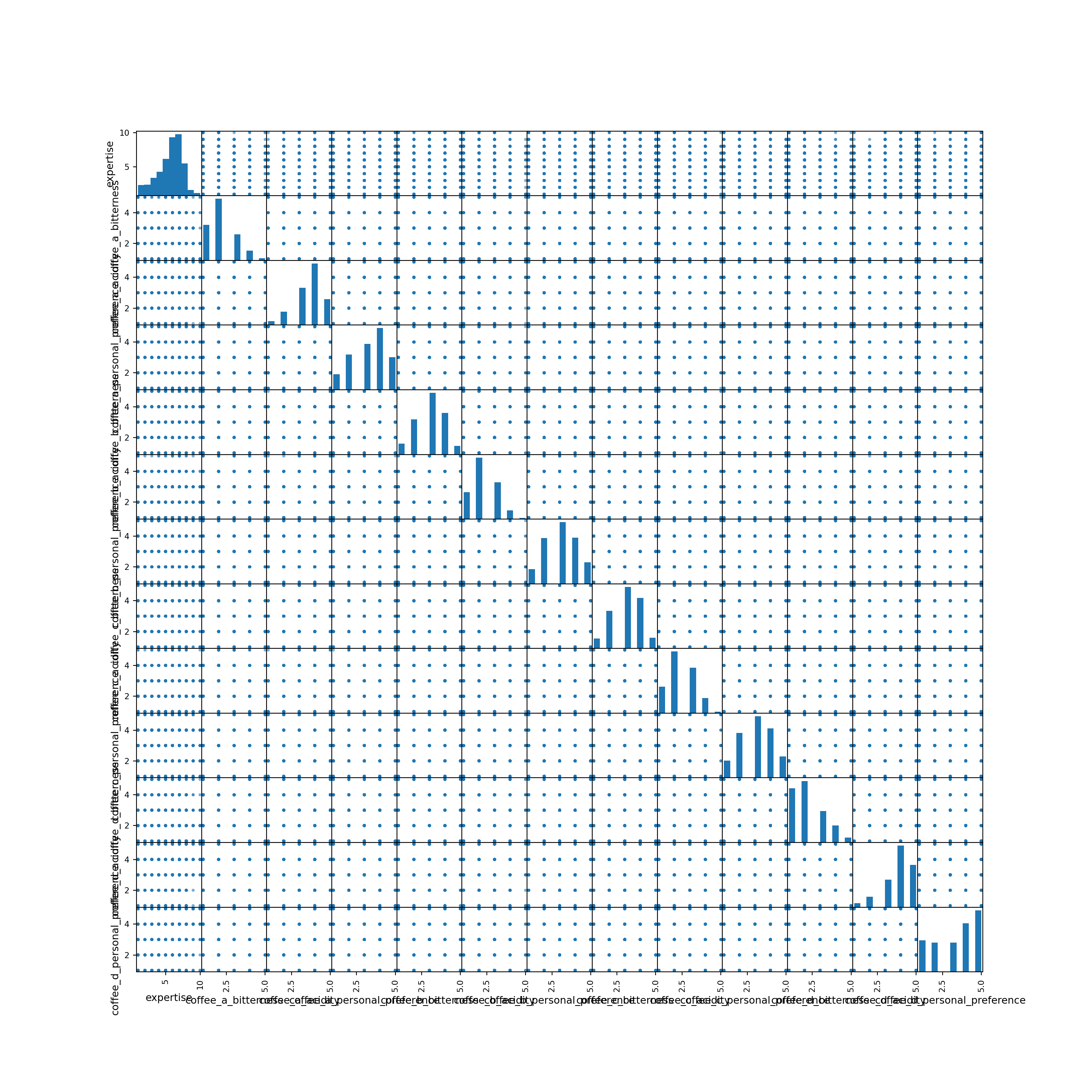
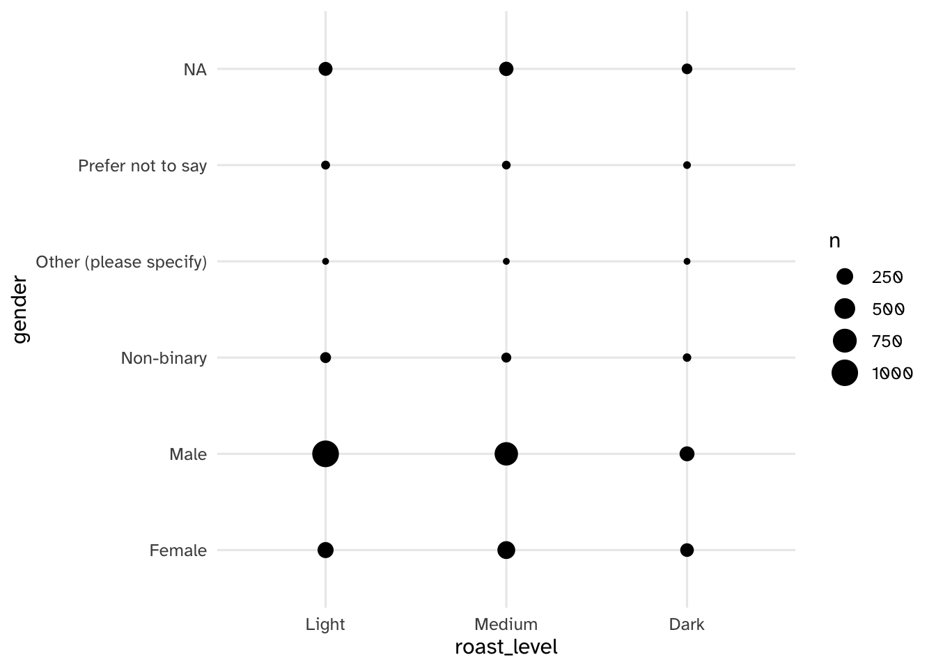
Your turn: Examine the distribution of roast/gender and roast/cups. Describe the patterns you see and anything that is of particular interest given the model we will estimate.
coffee_train |>
  filter(roast_level %in% c("Dark", "Medium", "Light")) |>
  mutate(
    roast_level = factor(roast_level, levels = c("Light", "Medium", "Dark")),
    cups = fct(cups) |>
      fct_relevel("Less than 1", "1", "2", "3", "4", "More than 4")
  ) |>
  ggplot(mapping = aes(x = roast_level, y = cups)) +
  geom_count()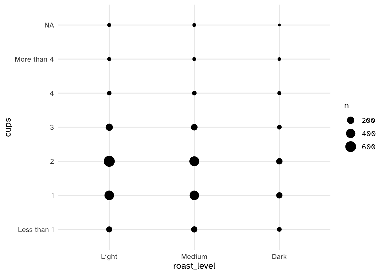
coffee_train |>
  filter(roast_level %in% c("Dark", "Medium", "Light")) |>
  mutate(
    roast_level = factor(roast_level, levels = c("Light", "Medium", "Dark")),
    cups = fct(cups) |>
      fct_relevel("Less than 1", "1", "2", "3", "4", "More than 4")
  ) |>
  ggplot(mapping = aes(x = roast_level, y = cups)) +
  geom_bin2d() +
  scale_fill_continuous_sequential(limits = c(0, NA))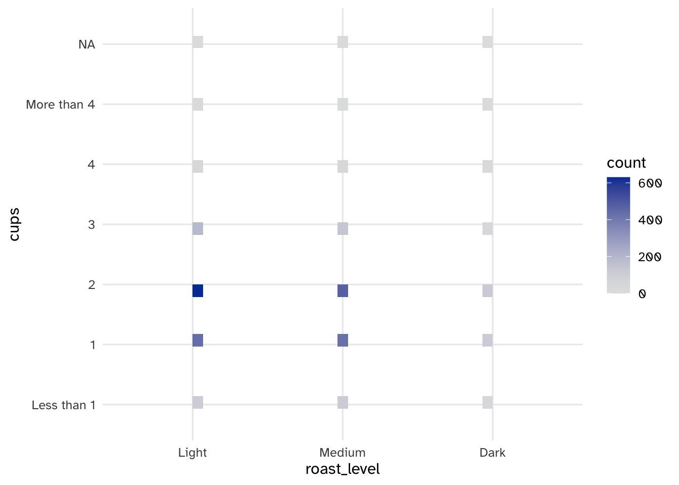
# Filter and prepare data
coffee_filtered = coffee_train[
    coffee_train['roast_level'].isin(['Dark', 'Medium', 'Light'])
].copy()

# Set roast_level as ordered categorical
coffee_filtered['roast_level'] = pd.Categorical(
    coffee_filtered['roast_level'],
    categories=['Light', 'Medium', 'Dark'],
    ordered=True
)

# Create the plot
(ggplot(coffee_filtered) +
  geom_count(aes(x='roast_level', y='gender'))).show()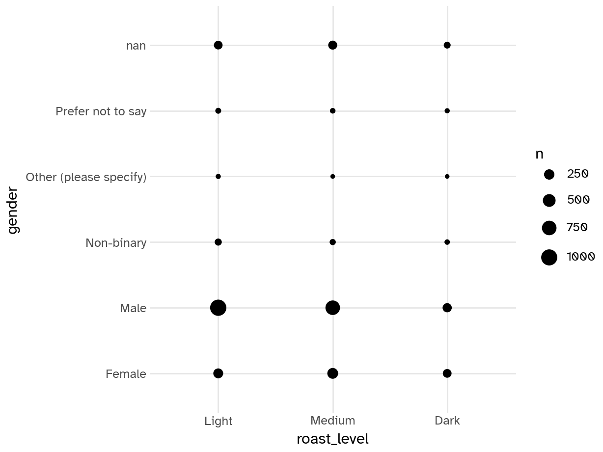
# Filter and prepare data
coffee_filtered = coffee_train[
    coffee_train['roast_level'].isin(['Dark', 'Medium', 'Light'])
].copy()

# Set both categorical variables with proper ordering
coffee_filtered['roast_level'] = pd.Categorical(
    coffee_filtered['roast_level'],
    categories=['Light', 'Medium', 'Dark'],
    ordered=True
)

coffee_filtered['cups'] = pd.Categorical(
    coffee_filtered['cups'],
    categories=["Less than 1", "1", "2", "3", "4", "More than 4"],
    ordered=True
)

# Plot 1: geom_count
(ggplot(coffee_filtered) +
  geom_count(aes(x='roast_level', y='cups'))).show()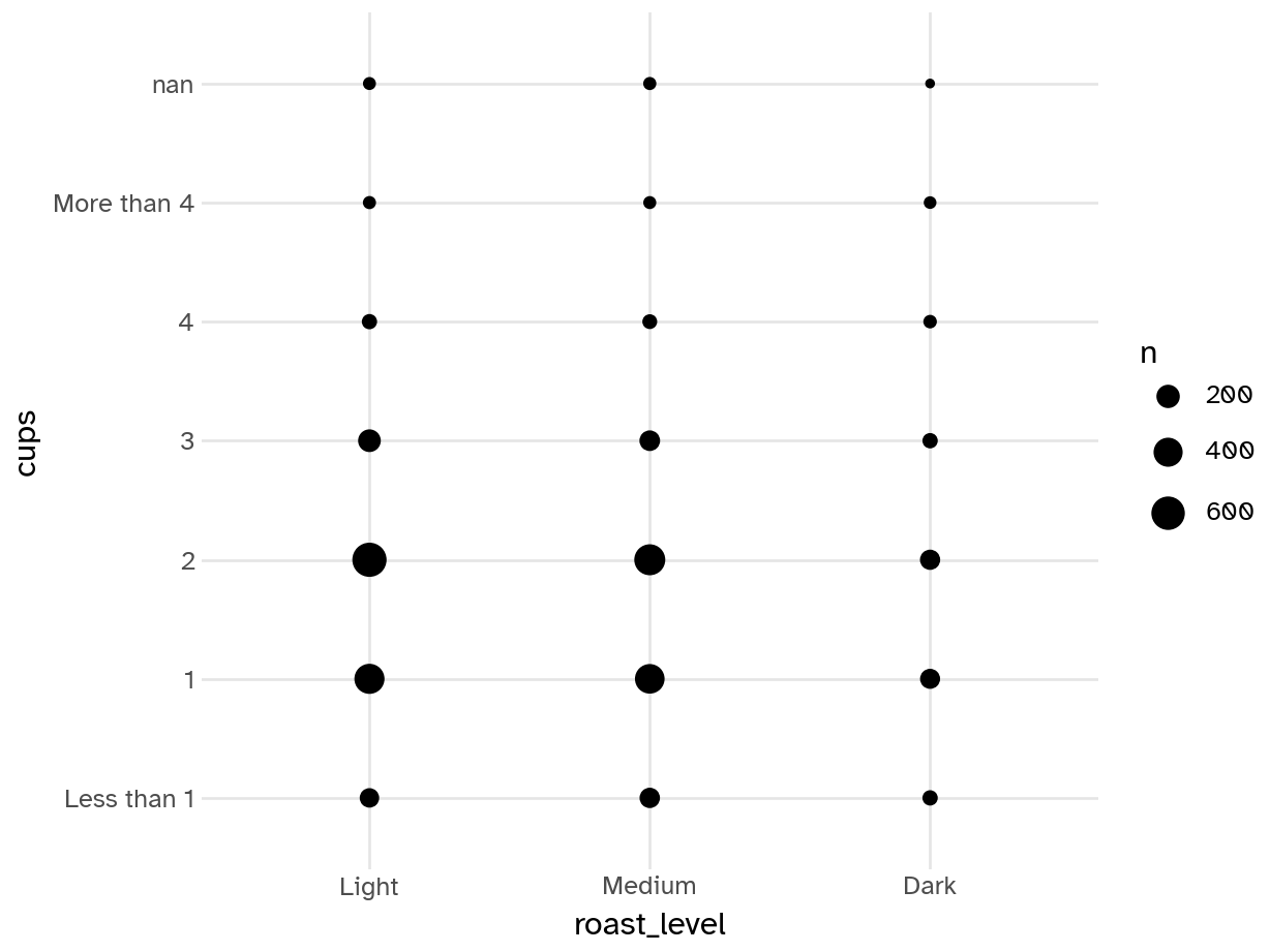
# Plot 2: geom_bin2d
(ggplot(coffee_filtered) +
  geom_bin2d(aes(x='roast_level', y='cups'))).show()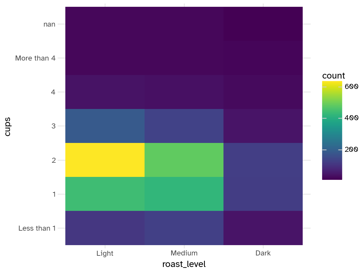
Add response here.
1-2 cups of light and medium roast are the most popular combinations. Everything else is significantly underrepresented. This could be a problem for the model if we don’t have enough data to make accurate predictions for these categories.
Acknowledgments
- Python examples are adapted from the R code and translated with support from Anthropic Claude 4 Sonnet.
NoteSession information
sessioninfo::session_info()─ Session info ───────────────────────────────────────────────────────────────
setting value
version R version 4.5.1 (2025-06-13)
os macOS Tahoe 26.0
system aarch64, darwin20
ui X11
language (EN)
collate C.UTF-8
ctype C.UTF-8
tz America/New_York
date 2025-09-26
pandoc 3.6.3 @ /Applications/Positron.app/Contents/Resources/app/quarto/bin/tools/aarch64/ (via rmarkdown)
quarto 1.8.24 @ /Applications/quarto/bin/quarto
─ Packages ───────────────────────────────────────────────────────────────────
! package * version date (UTC) lib source
P archive 1.1.12 2025-03-20 [?] CRAN (R 4.5.0)
P backports 1.5.0 2024-05-23 [?] RSPM (R 4.5.0)
P base64enc 0.1-3 2015-07-28 [?] RSPM (R 4.5.0)
P bit 4.6.0 2025-03-06 [?] RSPM (R 4.5.0)
P bit64 4.6.0-1 2025-01-16 [?] RSPM (R 4.5.0)
P broom * 1.0.9 2025-07-28 [?] RSPM (R 4.5.0)
P class 7.3-23 2025-01-01 [?] CRAN (R 4.5.1)
P cli 3.6.5 2025-04-23 [?] RSPM (R 4.5.0)
P codetools 0.2-20 2024-03-31 [?] CRAN (R 4.5.1)
P colorspace * 2.1-1 2024-07-26 [?] RSPM (R 4.5.0)
P crayon 1.5.3 2024-06-20 [?] RSPM (R 4.5.0)
P data.table 1.17.8 2025-07-10 [?] RSPM (R 4.5.0)
P dials * 1.4.1 2025-07-29 [?] RSPM
P DiceDesign 1.10 2023-12-07 [?] RSPM (R 4.5.0)
P digest 0.6.37 2024-08-19 [?] RSPM (R 4.5.0)
P dplyr * 1.1.4 2023-11-17 [?] RSPM (R 4.5.0)
P evaluate 1.0.4 2025-06-18 [?] RSPM (R 4.5.1)
P farver 2.1.2 2024-05-13 [?] RSPM (R 4.5.0)
P fastmap 1.2.0 2024-05-15 [?] RSPM (R 4.5.0)
P forcats * 1.0.0 2023-01-29 [?] RSPM (R 4.5.0)
P foreach 1.5.2 2022-02-02 [?] RSPM
P furrr 0.3.1 2022-08-15 [?] RSPM
P future 1.67.0 2025-07-29 [?] RSPM
P future.apply 1.20.0 2025-06-06 [?] RSPM
P generics 0.1.4 2025-05-09 [?] RSPM (R 4.5.0)
P GGally * 2.3.0 2025-07-18 [?] RSPM
P ggcorrplot * 0.1.4.1 2023-09-05 [?] RSPM
P ggplot2 * 4.0.0 2025-09-11 [?] RSPM
P ggstats 0.10.0 2025-07-02 [?] RSPM
P globals 0.18.0 2025-05-08 [?] RSPM
P glue 1.8.0 2024-09-30 [?] RSPM (R 4.5.0)
P gower 1.0.2 2024-12-17 [?] RSPM
P GPfit 1.0-9 2025-04-12 [?] RSPM (R 4.5.0)
P gtable 0.3.6 2024-10-25 [?] RSPM (R 4.5.0)
P hardhat 1.4.1 2025-01-31 [?] RSPM
P here 1.0.1 2020-12-13 [?] RSPM (R 4.5.0)
P hms 1.1.3 2023-03-21 [?] RSPM (R 4.5.0)
P htmltools 0.5.8.1 2024-04-04 [?] RSPM (R 4.5.0)
P htmlwidgets 1.6.4 2023-12-06 [?] RSPM (R 4.5.0)
P infer * 1.0.9 2025-06-26 [?] RSPM
P ipred 0.9-15 2024-07-18 [?] RSPM
P iterators 1.0.14 2022-02-05 [?] RSPM
P jsonlite 2.0.0 2025-03-27 [?] RSPM (R 4.5.0)
P knitr 1.50 2025-03-16 [?] RSPM (R 4.5.0)
P labeling 0.4.3 2023-08-29 [?] RSPM (R 4.5.0)
P lattice 0.22-7 2025-04-02 [?] CRAN (R 4.5.1)
P lava 1.8.1 2025-01-12 [?] RSPM
P lhs 1.2.0 2024-06-30 [?] RSPM (R 4.5.0)
P lifecycle 1.0.4 2023-11-07 [?] RSPM (R 4.5.0)
P listenv 0.9.1 2024-01-29 [?] RSPM
P lubridate * 1.9.4 2024-12-08 [?] RSPM (R 4.5.0)
P magrittr 2.0.3 2022-03-30 [?] RSPM (R 4.5.1)
P MASS 7.3-65 2025-02-28 [?] CRAN (R 4.5.1)
P Matrix 1.7-3 2025-03-11 [?] CRAN (R 4.5.1)
P modeldata * 1.5.0 2025-07-31 [?] RSPM
P nnet 7.3-20 2025-01-01 [?] CRAN (R 4.5.1)
P parallelly 1.45.1 2025-07-24 [?] RSPM
P parsnip * 1.3.2 2025-05-28 [?] RSPM
P pillar 1.11.0 2025-07-04 [?] RSPM (R 4.5.1)
P pkgconfig 2.0.3 2019-09-22 [?] RSPM (R 4.5.0)
P plyr 1.8.9 2023-10-02 [?] RSPM (R 4.5.0)
P png 0.1-8 2022-11-29 [?] RSPM (R 4.5.0)
P prodlim 2025.04.28 2025-04-28 [?] RSPM
P purrr * 1.1.0 2025-07-10 [?] RSPM (R 4.5.0)
P R6 2.6.1 2025-02-15 [?] RSPM (R 4.5.0)
P RColorBrewer 1.1-3 2022-04-03 [?] RSPM (R 4.5.0)
P Rcpp 1.1.0 2025-07-02 [?] RSPM (R 4.5.0)
P readr * 2.1.5 2024-01-10 [?] RSPM (R 4.5.0)
P recipes * 1.3.1 2025-05-21 [?] RSPM
renv 1.1.5 2025-07-24 [1] RSPM (R 4.5.0)
P repr 1.1.7 2024-03-22 [?] RSPM
P reshape2 1.4.4 2020-04-09 [?] RSPM (R 4.5.0)
P reticulate * 1.43.0 2025-07-21 [?] CRAN (R 4.5.0)
P rlang 1.1.6 2025-04-11 [?] RSPM (R 4.5.0)
P rmarkdown 2.29 2024-11-04 [?] RSPM
P rpart 4.1.24 2025-01-07 [?] CRAN (R 4.5.1)
P rprojroot 2.1.0 2025-07-12 [?] RSPM (R 4.5.0)
P rsample * 1.3.1 2025-07-29 [?] RSPM
P rstudioapi 0.17.1 2024-10-22 [?] RSPM (R 4.5.0)
P S7 0.2.0 2024-11-07 [?] RSPM (R 4.5.0)
P scales * 1.4.0 2025-04-24 [?] RSPM (R 4.5.0)
P sessioninfo 1.2.3 2025-02-05 [?] RSPM (R 4.5.0)
P skimr * 2.2.1 2025-07-26 [?] RSPM
P stringi 1.8.7 2025-03-27 [?] RSPM (R 4.5.0)
P stringr * 1.5.1 2023-11-14 [?] RSPM (R 4.5.1)
P survival 3.8-3 2024-12-17 [?] CRAN (R 4.5.1)
P tibble * 3.3.0 2025-06-08 [?] RSPM (R 4.5.0)
P tidymodels * 1.3.0 2025-02-21 [?] RSPM
P tidyr * 1.3.1 2024-01-24 [?] RSPM (R 4.5.0)
P tidyselect 1.2.1 2024-03-11 [?] RSPM (R 4.5.0)
P tidyverse * 2.0.0 2023-02-22 [?] RSPM (R 4.5.0)
P timechange 0.3.0 2024-01-18 [?] RSPM (R 4.5.0)
P timeDate 4041.110 2024-09-22 [?] RSPM
P tune * 1.3.0 2025-02-21 [?] RSPM
P tzdb 0.5.0 2025-03-15 [?] RSPM (R 4.5.0)
P utf8 1.2.6 2025-06-08 [?] RSPM (R 4.5.0)
P vctrs 0.6.5 2023-12-01 [?] RSPM (R 4.5.0)
P visdat * 0.6.0 2023-02-02 [?] RSPM
P vroom 1.6.5 2023-12-05 [?] RSPM (R 4.5.1)
P withr 3.0.2 2024-10-28 [?] RSPM (R 4.5.0)
P workflows * 1.2.0 2025-02-19 [?] RSPM
P workflowsets * 1.1.1 2025-05-27 [?] RSPM
P xfun 0.52 2025-04-02 [?] RSPM (R 4.5.1)
P yaml 2.3.10 2024-07-26 [?] RSPM (R 4.5.0)
P yardstick * 1.3.2 2025-01-22 [?] RSPM
[1] /Users/bcs88/Projects/info-4940/course-site/renv/library/macos/R-4.5/aarch64-apple-darwin20
[2] /Users/bcs88/Library/Caches/org.R-project.R/R/renv/sandbox/macos/R-4.5/aarch64-apple-darwin20/4cd76b74
* ── Packages attached to the search path.
P ── Loaded and on-disk path mismatch.
─ Python configuration ───────────────────────────────────────────────────────
python: /Users/bcs88/Projects/info-4940/course-site/.venv/bin/python
libpython: /Users/bcs88/.local/share/uv/python/cpython-3.13.6-macos-aarch64-none/lib/libpython3.13.dylib
pythonhome: /Users/bcs88/Projects/info-4940/course-site/.venv:/Users/bcs88/Projects/info-4940/course-site/.venv
virtualenv: /Users/bcs88/Projects/info-4940/course-site/.venv/bin/activate_this.py
version: 3.13.6 (main, Aug 14 2025, 16:07:26) [Clang 20.1.4 ]
numpy: /Users/bcs88/Projects/info-4940/course-site/.venv/lib/python3.13/site-packages/numpy
numpy_version: 2.3.2
NOTE: Python version was forced by VIRTUAL_ENV
──────────────────────────────────────────────────────────────────────────────