import polars as pl
import polars.selectors as cs
import seaborn as sbn
import matplotlib.pyplot as plt

# Make the graphs a bit prettier, and bigger
plt.style.use('ggplot')
plt.rcParams['figure.figsize'] = (15, 5)

print(pl.__version__)1.6.01.1 Reading data from a csv file
You can read data from a CSV file using the read_csv function. By default, it assumes that the fields are comma-separated.
We're going to be looking some cyclist data from Montréal. Here's the original page (in French), but it's already included in this repository. We're using the data from 2012.
This dataset is a list of how many people were on 7 different bike paths in Montreal, each day.
broken_df = pl.read_csv('../data/bikes.csv',encoding = "ISO-8859-1")
broken_df.head(3)| Date;Berri 1;Brébeuf (données non disponibles);Côte-Sainte-Catherine;Maisonneuve 1;Maisonneuve 2;du Parc;Pierre-Dupuy;Rachel1;St-Urbain (données non disponibles) |
|---|
| str |
| "01/01/2012;35;;0;38;51;26;10;1… |
| "02/01/2012;83;;1;68;153;53;6;4… |
| "03/01/2012;135;;2;104;248;89;3… |
You'll notice that this is totally broken! read_csv has a bunch of options that will let us fix that, though. Here we'll
- change the column separator to a
; - Set the encoding to
'latin1'(the default is'utf8') - Attempt to parse all date columns
- Explicitly set the datatype of two non-populated columns in the CSV sheet
fixed_df = pl.read_csv('../data/bikes.csv',
                       separator=';',
                       encoding='latin1',
                       try_parse_dates=True,
                       schema_overrides={'Brébeuf (données non disponibles)': pl.Int64,
                               'St-Urbain (données non disponibles)': pl.Int64}
)
fixed_df.head(3)| Date | Berri 1 | Brébeuf (données non disponibles) | Côte-Sainte-Catherine | Maisonneuve 1 | Maisonneuve 2 | du Parc | Pierre-Dupuy | Rachel1 | St-Urbain (données non disponibles) |
|---|---|---|---|---|---|---|---|---|---|
| date | i64 | i64 | i64 | i64 | i64 | i64 | i64 | i64 | i64 |
| 2012-01-01 | 35 | null | 0 | 38 | 51 | 26 | 10 | 16 | null |
| 2012-01-02 | 83 | null | 1 | 68 | 153 | 53 | 6 | 43 | null |
| 2012-01-03 | 135 | null | 2 | 104 | 248 | 89 | 3 | 58 | null |
1.2 Selecting a column
When you read a CSV, you get a kind of object called a DataFrame, which is made up of rows and columns. You get columns out of a DataFrame the same way you get elements out of a dictionary.
Here's an example:
fixed_df['Berri 1']| Berri 1 |
|---|
| i64 |
| 35 |
| 83 |
| 135 |
| 144 |
| 197 |
| … |
| 2405 |
| 1582 |
| 844 |
| 966 |
| 2247 |
1.3 Plotting a column
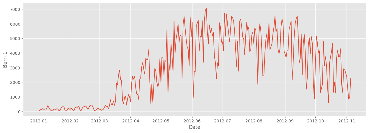
We can see that, unsurprisingly, not many people are biking in January, February, and March,
sbn.lineplot(fixed_df, x='Date', y='Berri 1')<Axes: xlabel='Date', ylabel='Berri 1'>
We can also plot all the columns just as easily. We'll make it a little bigger, too. You can see that it's more squished together, but all the bike paths behave basically the same -- if it's a bad day for cyclists, it's a bad day everywhere.
melt_df = fixed_df.unpivot(index='Date', variable_name='trail', value_name='distance')

with plt.rc_context({'figure.figsize': (15, 10)}):
    sbn.lineplot(melt_df, x='Date', y='distance', hue='trail')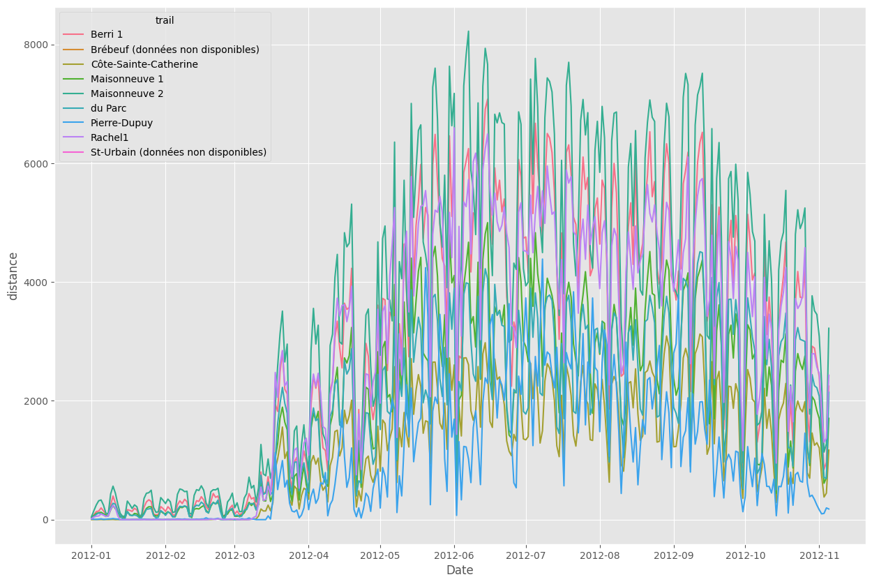
1.4 Putting all that together
Here's the code we needed to write do draw that graph, all together:
fixed_df = pl.read_csv('../data/bikes.csv', separator=';', encoding='latin1', try_parse_dates=True)
sbn.lineplot(fixed_df, x='Date', y='Berri 1')
<Axes: xlabel='Date', ylabel='Berri 1'>